Print ISSN: 2288-4637 / Online ISSN 2288-4645 doi:10.13106/jafeb.2021.vol8.no5.0583
Dynamic Impact of Macroeconomic Variables on the Ecological Footprint in Malaysia: Testing EKC and PHH*
Mahmood MEHRAAEIN1, Rafia AFROZ2, Mehe Zebunnesa RAHMAN3, Md MUHIBBULLAH4
Received: September 10, 2020 Revised: March 06, 2021 Accepted: April 15, 2021
Abstract
The objective of this paper is to investigate the impact of economic growth (per capita real GDP), the square of per capita real GDP, energy use, financial development (FD), and foreign direct investment (FDI) on ecological footprint (EF) in the case of Malaysia over the period 1971–2014, by employing the ARDL approach. The long-run results revealed that economic growth has a significant positive impact on the ecological footprint and it implies that the economic growth deteriorates the environmental quality in Malaysia. Conversely, the square of GDP showed a negative and significant impact on the EF in the long run. As the coefficient of GDP in our study is positive and statistically significant while the coefficient of squared GDP is negatively significant, thus, this study supports the presence of the environmental Kuznets curve (EKC) hypothesis in the case of Malaysia. Furthermore, the result indicates that FDI has a positive and significant impact on the EF in the long run, which means a rise in FDI will enhance the environmental pollution level. Thus, it confirms the pollution haven hypothesis. Hence, it suggests that Malaysia imposes stricter environmental policies. Further, FDI and FD are causing GDP in Malaysia, but through increasing EF.
Keywords: FDI, EKC, Pollution Haven Hypothesis, Energy Consumption JEL Classification Code: C22, E01, F18, P18, Q42
countries. The country’s Gross Domestic Product (GDP) was RM43,086 in 2018, which is around USD10,043, and the steady increase in GDP was 4.5 percent in the same year (Department of Statistics, Malaysia, 2019). During the past decades, Malaysia has suffered from an ecological deficit, implying that the Ecological Footprint (EF) in Malaysia is larger than that of the biocapacity. It means the human activities deteriorate more the environmental quality by creating waste, polluting air and water, emitting GHGs, deforesting, and reducing the natural sources than the ability of the earth to absorb the waste and produce the resources (Shahbaz et al., 2013; Gill et al., 2019; Ahmed et al., 2019). For this reason, environmental pollution is now increasingly recognized as a major threat to social and economic development and even to human survival. Failure to overcome environmental problems or to preserve a healthy environment will accelerate environmental degradation.
In addition, Malaysia’s economy grew by 4.2 percent in 2016, while energy demand was projected to rise by around 6 percent annually (Energy Commission Malaysia, 2017).
It should be noted that the key factors contributing positively to environmental pollution are economic development and energy use (Bekhet & Othman 2018; Saboori et al., 2012;
Destek & Sarkodie 2019). This has already been observed in Malaysia (Shahbaz et al., 2013; Gul et al., 2015); and in
*Acknowledgements:
1 The authors would like to acknowledge the P-RIGS funding from “Digital Development, Economics Growth. Environmental Sustainability and Population Health in Malaysia: Applying Response Surfaces for the F-test of cointegration model”
(Ref no: P-RIGS18-006-006).
1 First Author. Assistant Professor, Department of Banking and Business, Faculty of Economics and Management Sciences, Baghlan University, Afghanistan.
Email: [email protected]
2 Corresponding Author. Associate Professor, Department of Economics, Faculty of Economics and Management Sciences, International Islamic University Malaysia, Malaysia [Postal Address:
53100 Jalan Gombak, Kuala Lumpur, Malaysia]
Email: [email protected]
3 Assistant Professor, Department of Management, North South University, Dhaka, Bangladesh.
4 Ph.D. Candidate, Department of Economics, Faculty of Economics and Management Sciences, International Islamic University Malaysia, Malaysia. Email: [email protected]
© Copyright: The Author(s)
This is an Open Access article distributed under the terms of the Creative Commons Attribution Non-Commercial License (https://creativecommons.org/licenses/by-nc/4.0/) which permits unrestricted non-commercial use, distribution, and reproduction in any medium, provided the original work is properly cited.
1. Introduction
Among the Association of Southeast Asian Nations (ASEAN) countries, Malaysia is one of the fastest developing
other countries (Sarkodie & Ozturk, 2020; Mikayilov et al., 2018; Balsalobre-Lorente et al., 2018; Magazzino & Cerulli, 2019). For electricity generation, Malaysia relies mainly on 5 percent of fossil fuel consumption for hydro and other forms of renewable energy sources, 42 percent for natural gas, and 53 percent for coal (WEMO, 2017).
Due to the high fossil fuel energy consumption, CO2 emissions have risen proportionately and the position of Malaysia is even more susceptible to climate change (Ahmed et al., 2019; Suki et al., 2020; Destek & Sarkodia, 2019).
Since 2000, Malaysia has been losing an average of 140,200 hectares of its forests or 0.65 percent of its total forest area per year. As a consequence, the biodiversity of Malaysia is declining (Bekhet & Othman, 2018). Hence, more than 140%
increase in ecological footprint has been observed during the period of 1971 to 2014 in Malaysia, whereas, the availability of natural resources has declined by beyond 50 percent, causing an ecological deficiency of 85 percent. Therefore, the country is amongst those nations that consume more natural resources than they possess (Begum et al., 2009).
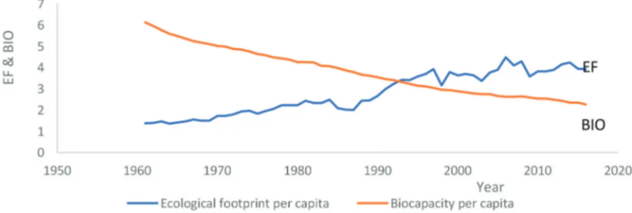
A consistent situation of ecological deficiency contributes to a more accelerated utilization of renewable resources, the depletion of ecological reserves, and even the collapse of the ecosystem (Ulucak & Bilgili, 2018). The EF in Malaysia is 3.9 global hectares per capita in 2019 (Global footprint network, 2020). This is twice the sum of biocapacity on the planet. Malaysia is ranked 35th in the world according to EF gha (global hectares) per capita and it was ranked 13th for the fishing industry and the ecological footprint is above the global average. Figure 1 clearly depicts that Malaysia had an ecological surplus (ecological reserve) from 1961 to 1991 while in the year 1992 it had ecological balance, which implies the equality in ecological footprint and biocapacity at 3.31 ecological footprint per person.
Since 1993 until now, Malaysia has an ecological deficit, which means that the EF of it exceeds biocapacity. Qatar, Luxembourg, UAE, Bahrain, Kuwait, and the USA have
the highest EF per capita while Afghanistan, Yemen, Haiti, Congo, and Malawi have the lowest EF per person in the world. As an example, Qatar has the highest EF per capita in 2019, which is 14.4, and Afghanistan has the lowest EF per capita in that year, which is 0.7 (Global footprint network, 2020). Malaysia has a Happy World Index Ranking of 30.3 and ranks 46th out of all the surveyed countries (Happy Planet Index, 2020). Besides this, climate change is expected to increase mean annual temperature and the risk of heat- related medical conditions. It can also cause cardiovascular and respiratory diseases. It increases the medical expenditure of the people in the society and reduces their productivity in the workplace. In Malaysia, it is estimated that a reduction in air pollutant could prevent 5,900 premature deaths attributed to outdoor air pollution per year, from 2030 onwards (WHO, 2020; Afroz et al., 2020). To the best of our knowledge, no study has been done in Malaysia to explore the validity of the environmental Kuznets curve (EKC) hypothesis using the ARDL approach by considering the EF, energy consumption, FDI, and FD together in a model.
2. Literature Review
The idea of the Kuznets curve was first suggested by Simon Kuznets in his presentation at the American Economic Association in 1954 and in his paper published in 1955 in the Journal of Economic Perspectives. Kuznets claimed and showed proof that the connection between economic prosperity and inequalities persisted. The association between the Kuznets has been extended to environmental indices such as emissions of GHGs and other contaminants. The relationship explains that the amount of environmental pollution factors rises to some degree and, then declines as an economy progresses. This suggests that, eventually, an increasing economy will hit a threshold where stronger environmental and economic controls and higher expenditure in renewable energies can help battle pollution.
Figure 1: Ecological Footprint and Biocapacity of Malaysia from 1961–2016 Source: GFN, 2020
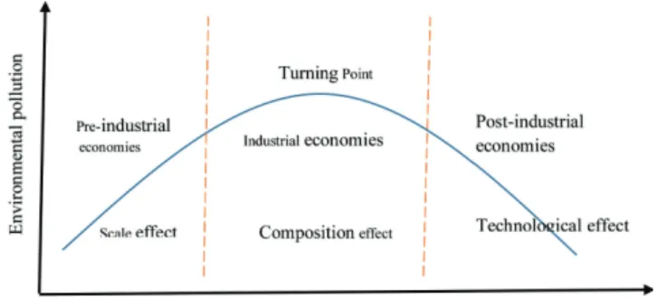
This hypothesis is popularized by the study of Grossman and Kruegers (1991) as a result of their analysis of Sulphur Dioxide and smoke’s relationship to income. Its results found that the SO2 and the income had a positive association until the point in which the pattern transformed into a negative correlation. The EKC hypothesis was eventually expanded, not only to include SO2, but also other emission forms (Yin et al., 2015). Subsequently, many studies supported this relationship such as Shafik and Bandyopadhyay (1992) and Panayotou (1993), who called this inverted U-shaped relationship EKC. Grossman and Krueger (1991) emphasize how economic growth affects the environmental quality by three modes, namely, scale effect, technological effect, and composition effect.
Figure 2 shows these three effects. The scale effect reflects the original negative environmental effects of economic growth. In brief, economic development results in higher production and hence environmental degradation;
because higher output often means higher inputs, and inputs are meanly consumption of natural resources (Grossman &
Krueger, 1991). So, consumption of natural resource leads to environmental degradations and usage of more outputs pollute more the environment.
Technological effect catches changes in efficiency and adaptation to cleaner technology, contributing to improving the environmental standards. The composition effect is a shift in the formation of products and services as the economy undergoes a systemic transition from a manufacturing society to a more service-based system (Álvarez-Herránz et al., 2017). So, this transition in production may have a positive effect on environmental quality.
3. Data Descriptions
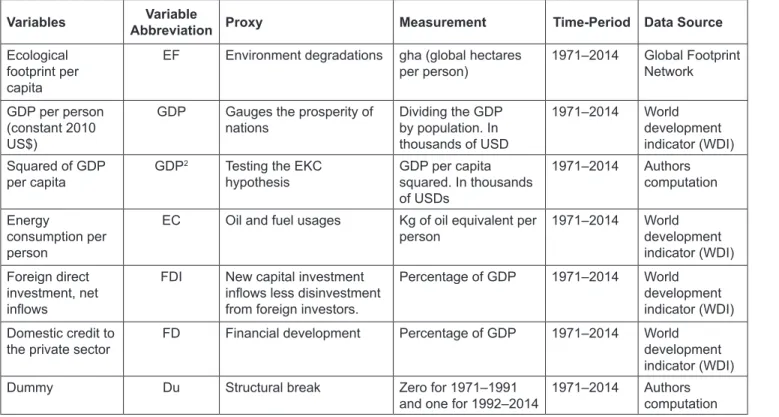
This study includes an annual series data from 1971 to 2014, which are taken from reliable sources such as the global footprint network and the World development indicator (WDI). The dependent variable is the ecological
footprint (EF) measured as gha (global hectares per person). The explanatory variables are Gross Domestic Product (GDP) measured as GDP per person (constant 2010 US$) in thousands of USD, the square of GDP, energy consumption (EC) measured as kg of oil equivalent per capita, foreign direct investment (FDI) measured as the net inflows percentage of GDP, and financial development (FD) measured as domestic credit to private sector % of GDP.
The description of the variables and sources of data are displayed in Table 1.
4. Construction of the Model
This study explores the impact of economic growth (GDP per capita), foreign direct investment (FDI), energy consumption (EC), and financial development (FD) on the ecological footprint (EF) to test the validity of the EKC hypothesis in the case of Malaysia. So, this study defines ecological footprint as a function of GDP, the square of GDP, energy consumption, foreign direct investments, and financial development for the period of 1971–2014.
We extract the empirical model based on the regular Cobb-Douglas production function, so our model is presented in the following equation (1):
Yt = F(Kt, ALt) (1) Where Yt represents output, Kt is capital land, and ALt shows effective labor. Since humankind is polluting the ecosystem because of its economic and other activities, and it affects ecological footprint so that the ecological footprint function can be represented as in the following equation (2):
EF = V (F(Yt)) (2)
Where v shows the impact rate of production activities on the EF. Even though all capital forms do not affect the EF, so the total capital can be split into two parts as in the following equation (3):
K = Ki + Kh (3)
Where Ki indicates capitals rising EF and Kh represents capitals not increasing EF. Hence, the part of capital, which increases EF is included in the function of EF as in the following equation (4):
EF = αKi(Yt) (4)
Equation (4) needs to be expanded with the inclusion of the important variables affecting EF to avoid omitted variable bias.
Figure 2: Environment Kuznets Curve Source: Panayotou (1993)
For testing the existence of the EKC hypothesis the conventional model uses GDP and square of GDP as regressors and we call it quadratic form. Some researchers used the cubic form of GDP to test the EKC hypothesis validity, although, a modern way to test the existence of the EKC hypothesis was proposed by Narayan (2010) and Al-Mulali et al. (2015). As in their studies, they compare the coefficients of the short run and long run of GDP with each other. If the elasticity (coefficient) of long-run GDP would be lower than the coefficient of short-run GDP, then they inferred that economic growth would contribute less to environmental degradation over time. Therefore, it validates the EKC hypothesis. Our study follows the conventional way to test the EKC hypothesis. So, following the work of Saboori and Sulaiman (2013), Mrabet and Alsamara (2016), Ali et al. (2017), Dogan et al. (2019), Nosheen et al. (2019), Gill et al. (2019), Bulut (2020), Ergun and Rivas (2020), Sarkodie and Ozturk (2020), the empirical equation to test the EKC hypothesis for this study is presented in quadratic form as in the following equation (5):
EF=F(GDP GDP, i2) (5) Where EF denotes ecological footprint per capita, GDP and GDP2 represents gross domestic product per capita, and the square of GDP, respectively. As we know various
forms of human activities impact environmental quality.
By including all variables into the model will increases the fit of the model and obtains the augmented model of equation (5) but eventually will decrease the degrees of freedom (Sarkodie & Ozturk, 2020). For this reason, this study is restricted to EC, FDI, and FD. This study uses time-series data for the period of 1971 to 2014 on the basis of data availability for the energy consumption variable.
In the linear equation form, the model in this study can be described as in the following equation (6):
EFt = (f GDP GDP EC FDI FDt, t2, t, t, t) (6) This model is non-linear therefore it transformed as the augmented Cobb-Douglas production function as Equation (7):
EFt 0GDP GDPt 1 t2 2EC FDI FD 23 t 4 t 5 t (7) All variables in equation (7) are transformed into natural logarithmic forms as in the following equation (8) to obtain direct elasticity and consistently reliable results. It also can reduce the multicollinearity problem and the coefficients easily can capture the variation effect of explanatory variables on the dependent variable, which is ecological footprint.
Table 1: Description of the Variables
Variables Variable
Abbreviation Proxy Measurement Time-Period Data Source
Ecological footprint per capita
EF Environment degradations gha (global hectares
per person) 1971–2014 Global Footprint Network GDP per person
(constant 2010 US$)
GDP Gauges the prosperity of
nations Dividing the GDP
by population. In thousands of USD
1971–2014 World development indicator (WDI) Squared of GDP
per capita GDP2 Testing the EKC
hypothesis GDP per capita
squared. In thousands of USDs
1971–2014 Authors computation Energy
consumption per person
EC Oil and fuel usages Kg of oil equivalent per
person 1971–2014 World
development indicator (WDI) Foreign direct
investment, net inflows
FDI New capital investment inflows less disinvestment from foreign investors.
Percentage of GDP 1971–2014 World development indicator (WDI) Domestic credit to
the private sector FD Financial development Percentage of GDP 1971–2014 World development indicator (WDI)
Dummy Du Structural break Zero for 1971–1991
and one for 1992–2014 1971–2014 Authors computation
Also, natural logarithms of variables stabilize the variance, linearize the nexus, induce the stationarity test (Lau et al., 2014), and reduce the possibility of autocorrelation in the series (Bekhet & Othman, 2018).
LnEF LnGDP LnGDP LnEC
LnFDI LnFD
t t t t
t t t
0 1 2
2 3
4 5
(8)
Where, LnEFt, LnGDPt, LnGDPt2, LnECt, LnFDIt, and LnFDt, respectively, stand for the natural logarithm of ecological footprint, GDP per capita, the square of GDP, energy consumption, foreign direct investments, and financial development. Furthermore, εt represents error term, the parameters βi, i = 1, 2…5, are the coefficients of the regressors and represents the long-run elasticity of LnGDPt, LnGDPt2, LnECt, LnFDIt, and LnFDt respectively. The β0 is intercept and shows that when there is no change in other variables the emission is equal to this autonomous value.
The εt captures the impact of other variables that are not included in the model. The t at the end of variables indicates that all variables are time series data. The data for EF is taken from Global Footprint Network (2020). The data of GDP, FDI, and FD data are obtained from World Development Indicator, World Bank (2020).
According to the theory for the quadratic form of the model, the EKC hypothesis holds when the expected sign of β1 is positive and significant while the expected sign of β2 is negatively significant, which highlights the GDP growth will rise the environmental quality over time. According to the findings of researchers, we expect the sign of β3 to be positive because EC leads to an increase the environmental pollution. Moreover, the expected sign of β4 can be both positive and negative, relying upon the environmental regulation of the host countries towards the FDI inflows. In the case of flexible environmental regulations and pollution haven hypothesis the predicted sign of the β4 is positive while in the case of strict environmental regulations and pollution halo hypothesis, wexpect a negative sign for β4. Lastly, we expect both positive and negative signs for β5 relying upon the improvement level of the financial system in a country for the relationship between EF and FD.
5. Results and Discussion 5.1. The Stationarity Results
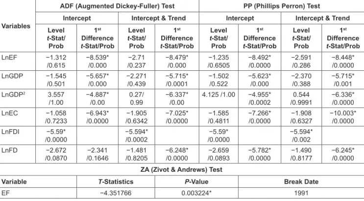
The results of Augmented Dickey-Fuller (ADF), Phillips Perron (PP), and Zivot & Andrews (ZA) unit root tests are displayed in Table 2 and the results confirm that EF,
Table 2: The Unit Root Tests Summary
Variables
ADF (Augmented Dickey-Fuller) Test PP (Phillips Perron) Test
Intercept Intercept & Trend Intercept Intercept & Trend Level
t-Stat/
Prob
1st Difference t-Stat/Prob
Level t-Stat/
Prob
1st Difference t-Stat/Prob
Level t-Stat/
Prob
1st Difference t-Stat/Prob
Level t-Stat/
Prob
1st Difference t-Stat/Prob
LnEF −1.312
/0.615 −8.539*
/0.000 −2.71
/0.237 −8.479*
/0.000 −1.235
/0.6505 −8.492*
/0.0000 −2.591
/0.286 −8.448*
/0.0000
LnGDP −1.545
/0.501 −5.657*
/0.000 −2.271
/0.439 −5.715*
/0.0001 −1.502
/0.522 −5.623*
/0.000 −2.370
/0.388 −5.715*
/0.001
LnGDP2 3.557
/1.00 −4.887*
/0.00 0.27/
0.99 −6.337*
/0.00 4.125 /1.00 −4.955*
/0.0002 0.544
/0.9991 −6.336*
/0.0000
LnEC −1.058
/0.7233 −6.943*
/0.0000 −1.905
/0.6342 −7.025*
/0.0000 −1.585
/0.4811 −7.266*
/0.0000 −1.908
/0.6327 −10.003*
/0.0000
LnFDI −5.59*
/0.0000 −5.594*
/0.0002 −5.59*
/0.0000 −5.594*
/0.002
LnFD −2.672
/0.0870 −2.341
/0.1646 −1.481
/0.8205 −6.248*
/0.0000 −2.659
/0.0893 −5.782*
/0.0000 −1.490
/0.8177 −6.245*
/0.0000 ZA (Zivot & Andrews) Test
Variable T-Statistics P-Value Break Date
EF −4.351766 0.003224* 1991
Note: *Represents a 1% level of significance.
GDP, EC, and FD are nonstationary at the level while they are stationary and integrated at their first difference. Only FDI is stationary at level, hence, it is integrated at order I(0). Therefore, this study shows a mixture of I(1) and I(0) of variables. Thus, it is recommended to use the ARDL approach for this study. The results of the stationarity tests reveal that there is no variable, that is integrated of order I(2).
Therefore, short-run and long-run estimation procedures can be conducted to examine whether there is long run and short run relationship among the variables. Moreover, the result of ZA unit root test reveals a structural break date in the year 1991 for the EF. The structural breaks in 1991 can be explained by the rapid growth of the economy and a sudden change of EF in that year. Hence, the structural break replicates that Malaysian economy has witnessed a major change after 1991. Therefore, a dummy variable is introduced to capture the sudden changes in 1991. According to the ZA unit root test, the EF shows a structural break in 1991. Figure 3 represents that EF has faced a sudden change in that year.
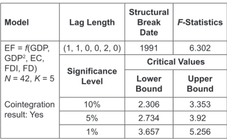
5.2 ARDL F-Bounds Test for Cointegration Results
The empirical outcome of the bounds test in Table 3 shows that the computed value of F-statistics is greater than the upper bound critical value at 1% significance level. The ARDL approach shows 3.06 and 4.14 critical values at 1% percent level for lower bound and upper bound, respectively. However, the estimated F-statistics is 6.302, which is higher than the upper bound. So, this study fails to reject the alternative hypothesis, which implies that cointegration exists among variables. Thus, all the variables (EF, GDP, GDP2, EC, FDI, and FD) are cointegrated in the model of this study. In the next step, ARDL model is conducted to find the estimated values
of the long run and short run coefficients since this study confirms the bounds test of cointegration and long-run relationship among variables.
5.3. Long-Run Results of ARDL Approach
The long-run results of the ARDL model are displayed in Table 4. The long-run results reveal that there is a significant and positive association between economic growth and EF, i.e., the economic growth is at the cost of environmental quality in Malaysia. If there occur 1%
increase in GDP per capita, it will cause an increase of 0.82% in EF in the long run in Malaysia. Conversely, the square of GDP shows a negative and significant impact on the EF in the long run. These findings seem to approve the quadratic relationship between economic growth and ecological footprint and imply that, in the initial phase of economic growth, the level of pollution increases in terms of ecological footprint. However, economic growth helps to minimize pollution after reaching the optimum level, which supports the EKC hypothesis in Malaysia.
Figure 3: ZA Unit Root Test for a Structural Break Date Source: Authors Computation
Table 3: Result of ARDL F-Bounds Test for Cointegration Model Lag Length Structural
Break
Date F-Statistics EF = f(GDP,
GDP2, EC, FDI, FD) N = 42, K = 5 Cointegration result: Yes
(1, 1, 0, 0, 2, 0) 1991 6.302 Significance
Level
Critical Values Lower
Bound Upper
Bound
10% 2.306 3.353
5% 2.734 3.92
1% 3.657 5.256
Table 4: Description of the Variables Depended Variable: Ln_EFt Variables Coefficients Std.
Error t-Statistics Prob
Ln_GDP 0.828 0.301 2.746 0.009***
Ln_GDP2 −4.01E−09 1.62E−09 −2.477 0.018***
Ln_EC 0.063 0.171 0.366 0.716
Ln_FDI 0.066 0.019 3.403 0.001***
Ln_FD −0.156 0.055 −2.823 0.008***
C −5.774 1.354 −4.262 0.000***
Note: ***1% level of significance, **5% level of significance.
This finding is in line with the results of many researchers in the case of Malaysia (Saboori et al., 2012; Lau et al., 2014;
Apergis & Ozturk, 2015; Ali et al., 2017; Bello et al., 2018;
Sinaga et al., 2019; Saudi et al., 2019; Gill et al., 2019;
Suki et al., 2020). The results of this study reflect the fact that by investing more in improving society and systemic transition from a manufacturing society to a more service- based economy, GDP growth can have a positive effect on the quality of the environment. Hence, this outcome supports the EKC hypothesis by suggesting that along with GDP growth, environmental standards are improved by the adaptation of cleaner technology and government pollution control policies.
To more extent, the results of this study indicate that FDI has a positive and significant impact on the EF in the long run in Malaysia. The coefficient of FDI concludes that 1% rise in FDI leads to an increase of ecological footprint by 0.06% in Malaysia. The finding of this study supports the PHH, which implies while FDI may encourage higher economic growth, higher industrial pollution and environmental degradation may also result.
This result is consistent with the findings of other studies such as Sabir et al. (2020), Baloch et al. (2019), Khan et al. (2020) and Murthy et al. (2021). This result shows the motive of some multinational companies (MNCs) that shift their industrial operations to developing nations to reduce the expense of environmental regulations in their home countries. This will make the environmental efficiency of certain host countries even worse. In this case, only encourage those FDI inflows that do not harm the environmental quality and which are environmental friendly projects.
Moreover, the negative and significant sign of FD coefficient indicates that, in the long run, it could help to reduce some part of the EF. Hence, in this way it can decrease the pollution level in Malaysia. The empirical findings suggest that if FD increases by 1%, EF will decrease by 0.15%. This result is supported by the findings of Ozturk and Acaravci (2013), Shahbaz et al. (2013), and Gill et al. (2019) for Malaysia; Aluko and Obalade (2020) for sub-Saharan Africa, Habib-Ur-Rahman et al. (2020) for Lithuania; Villanthenkodath and Arakkal (2020) for New Zealand, and Alzyadat (2021), Raggad (2020) for Saudi Arabia. The result point outs that the financial sector of Malaysia contributes to the improvement of environmental quality by supporting research and development, promoting cleaner technology adoption, and providing loans and funds for businesses to spend further on clean energy development and promoted energy- efficiency strategies in the last few years. In addition, the empirical outcome indicates that energy consumption has a positive impact on the ecological footprint in the long
run and it will contribute to environmental pollution in Malaysia, but it is not significant. Maybe because this study considers an aggregate form of energy consumption in the model and the significant effects of disaggregate energy consumption cancel out each other.
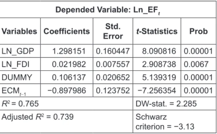
5.4. Short-Run Results of ARDL Approach
The short-run results and their diagnostics tests are displayed in Table 5. It shows that economic growth increases the ecological footprint in the short run and this finding is consistent with our long-run results. It indicates that an increase of 1% in the GDP per capita will rise EF by 1.29% in the short run, ceteris paribus. Moreover, FDI inflows have also a positive and significant impact on the EF in the short run, and the empirical short-run estimates that a 1% rise in the FDI inflows will lead to a 0.02% decline in the EF. In addition, the dummy variable, which takes account of the structural change in the dependent variable has a positive and significant impact on the EF in the short run. This reveals that the structural change in the economy of Malaysia has a positive effect on environmental pollution. Besides, EC and FD are insignificant in the short-run, which implies these variable do no impact on the EF in the short run.
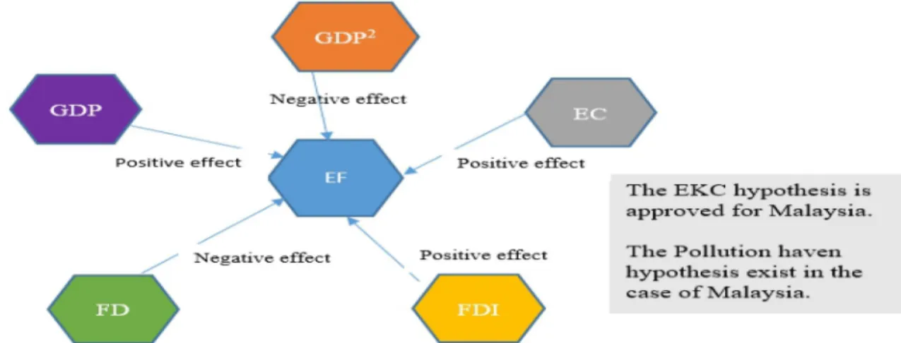
Most importantly, the coefficient of ECTt−1 is negative and statistically significant at the 1% level, which documents additional support of long-run cointegration among variables. The value of ECTt−1 is −0.897, which implies that 89% of disequilibrium in ecological footprint per capita due to previous years’ shocks converges back to the long-term equilibrium in the current year. For the quick understanding Figure 4 shows the estimated results of the ARDL approach.
It indicates the direct effect of each explanatory variables on the dependent variable. From this figure we can see the results of our model for the relationship of GDP, GDP2, EC, FDI, and FD with the EF.
Table 5: Estimated Short-Run Coefficients Depended Variable: Ln_EFt Variables Coefficients Std.
Error t-Statistics Prob LN_GDP 1.298151 0.160447 8.090816 0.00001 LN_FDI 0.021982 0.007557 2.908738 0.0067 DUMMY 0.106137 0.020652 5.139319 0.00001 ECMt−1 −0.897986 0.123752 −7.256354 0.00001
R2 = 0.765 DW-stat. = 2.285
Adjusted R2 = 0.739 Schwarz criterion = −3.13
6. Conclusion and Policy Implications
The economic growth and energy use due to the high fossil fuel energy consumption have risen the environmental pollution level in Malaysia (Bekhet & Othman 2018;
Destek & Sarkodie 2019). The continuation state of ecological deficit and environmental pollution can inflict devastating ecosystem problems. The conflictions of the findings in the previous studies about the EKC hypothesis and about the relationship between considered variables for this study in Malaysia, motivated us to address this problem.
The objective of this paper is to investigate the impact of per capita real GDP, the square of per capita real GDP, energy use, FD, and FDI on EC in the case of Malaysia over the period 1971–2014, by employing the ARDL approach. The ARDL bounds test fails to reject the alternative hypothesis, which implies that cointegration exists among variables.
The long-run results revealed that economic growth has a significant positive impact on the ecological footprint and it implies that the economic growth deteriorates the environmental quality in Malaysia. Conversely, the square of GDP showed a negative and significant impact on the EF in the long run. As the coefficient of GDP in our study is positive and statistically significant while the coefficient of squared GDP is negatively significant, thus, this study supports the presence of the EKC hypothesis in the case of Malaysia. The EKC curve turning point is computed to be outside of the range of the sample period. Furthermore, the result indicates that FDI has a positive and significant impact on the EF in the long run which means a rise in FDI will enhance the environmental pollution level. Thus, it confirms the pollution haven hypothesis. This could be because of weak environmental regulations. Hence, it suggests that Malaysia imposes stricter environmental policies.
In addition, the empirical outcome indicates that energy consumption has a positive impact on the ecological footprint in the long run and it will contribute to environmental pollution in Malaysia, but it is not significant. So, it is important for Malaysia to decline the use of conventional energy sources by investing in renewable energy sources such as solar, wind, and hydro. Furthermore, Malaysia should use its unexploited renewable energy sources and diversify its energy sources. Moreover, in order to increase public understanding of energy usages and environmental conservation some policies should be enforced. Besides, the country should rise the research and development for energy sector to improve energy efficiency. The result revealed that financial development increases the quality of environment. As it raises FDI inflows and enhances energy innovation through research and development, and offers loans. Therefore, financial system should offer loans and finance for eco-friendly projects and not allocate funds for environmental pollutions projects. Also, it is recommended that FD should facilitate financial support for eco-friendly activities at a minimum interest rate. The short-run results show that GDP per capita similar to the long run has a positive and significant impact on the EF.
Moreover, FDI inflows have a positive and significant impact on the EF in the short run. The pollutant industries add tariffs to the non-environmentally-friendly energy products, and subsidize clean industries. The government of Malaysia should increase Pigouvian tax gradually on the industries that creates externalities. It forces the industries to shift their production procedure to more clean energy usages. Finally, the country should increase the climate awareness among the citizens through print and electronic media. These policy implications are not limited to Malaysia, but it is also applicable to other emerging countries.
Figure 4: Estimated Result from ARDL Approach
So, the recommendation relying on the findings of this study could enable policymakers in Malaysia to have a pollution- free society. Similarly, other developing countries could make policies based on the results of this study that are the most suitable for improving the quality of their environments.
This research paper encountered some limitations. Firstly, the proxy of the variables differs in most of the studies and it causes to get different findings from the empirical results.
Also, the estimation is based on the macro variables. Thus, the unavailability of data on a regional scale constrains this study from going further. Secondly, the environmental pollution has various form of the proxy. For instance, CO2, SOx, NOx, EF, etc. This study used EF as a proxy to address environmental degradation. However, other proxies may receive different outcome for the objective of this study.
Therefore, future studies are encouraged to test the objective of this study with other proxies of the considered variables.
Thirdly, the time horizon of this study is limited to 2014, based on the data availability for energy consumption series.
So, it is suggested for further studies to collect latest data for their studies and also they can use the disaggregate form of the energy consumption for their studies.
References
Afroz, R., Muhibbullah, M., & Morshed, M. N. (2020). Impact of information and communication technology on economic growth and population health in Malaysia. Journal of Asian Finance, Economics and Business, 7(4), 155–162. https://doi.
org/10.13106/jafeb.2020.vol7.no4.155
Ahmed, Z., Wang, Z., Mahmood, F., Hafeez, M., & Ali, N. (2019).
Does globalization increase the ecological footprint? Empirical evidence from Malaysia. Environmental Science and Pollution Research, 26(18), 18565–18582. https://doi.org/10.1007/
s11356-019-05224-9
Ali, W., Abdullah, A., & Azam, M. (2017). Re-visiting the environmental Kuznets curve hypothesis for Malaysia: Fresh evidence from ARDL bounds testing approach. Renewable and Sustainable Energy Reviews, 77(9), 990–1000. https://doi.
org/10.1016/j.rser.2016.11.236
Al-Mulali, U., Solarin, S. A., & Ozturk, I. (2015). Investigating the presence of the environmental Kuznets curve (EKC) hypothesis in Kenya: an autoregressive distributed lag (ARDL) approach.
Natural Hazards, 80(3), 1729–1747. https://doi.org/10.1007/
s11069-015-2050-x
Aluko, O. A., & Obalade, A. A. (2020). Financial development and environmental quality in sub-Saharan Africa: Is there a technology effect? Science of the Total Environment, 747, 141515. https://doi.org/10.1016/j.scitotenv.2020.141515 Álvarez-Herránz, A., Balsalobre, D., Cantos, J. M., & Shahbaz, M.
(2017). Energy Innovations-GHG Emissions Nexus: Fresh Empirical Evidence from OECD Countries. Energy Policy, 101(October 2016), 90–100. https://doi.org/10.1016/j.
enpol.2016.11.030
Alzyadat, J. A. (2021). Sectoral banking credit facilities and non-oil economic growth in Saudi Arabia: application of the autoregressive distributed lag (ARDL). Journal of Asian Finance, Economics and Business, 8(2), 809–820. https://doi.
org/10.13106/JAFEB.2021.VOL8.NO2.0809
Apergis, N., & Ozturk, I. (2015). Testing environmental Kuznets curve hypothesis in Asian countries. Ecological Indicators, 52, 16–22. https://doi.org/10.1016/j.ecolind.2014.11.026
Baloch, M. A., Zhang, J., Iqbal, K., & Iqbal, Z. (2019). The effect of financial development on ecological footprint in BRI countries: evidence from panel data estimation. Environmental Science and Pollution Research, 26(6), 6199–6208. https://doi.
org/10.1007/s11356-018-3992-9
Balsalobre-Lorente, D., Shahbaz, M., Roubaud, D., & Farhani, S.
(2018). How economic growth, renewable electricity and natural resources contribute to CO2 emissions? Energy Policy, 113(11), 356–367. https://doi.org/10.1016/j.enpol.2017.10.050 Begum, R. A., Pereira, J. J., Jaafar, A. H., & Al-Amin, A. Q. (2009).
An empirical assessment of ecological footprint calculations for Malaysia. Resources, Conservation and Recycling, 53(10), 582–587. https://doi.org/10.1016/j.resconrec.2009.04.009 Bekhet, H. A., & Othman, N. S. (2018). The role of renewable
energy to validate dynamic interaction between CO2 emissions and GDP toward sustainable development in Malaysia.
Energy Economics, 72, 47–61. https://doi.org/10.1016/
j.eneco.2018.03.028
Bello, M. O., Solarin, S. A., & Yen, Y. Y. (2018). The impact of electricity consumption on CO2 emission, carbon footprint, water footprint and ecological footprint: The role of hydropower in an emerging economy. Journal of Environmental Management, 219, 218–230. https://doi.org/10.1016/
j.jenvman.2018.04.101
Bulut, U. (2020). Environmental sustainability in Turkey: an environmental Kuznets curve estimation for ecological footprint.
International Journal of Sustainable Development and World Ecology. https://doi.org/10.1080/13504509.2020.1793425 Department of Statistics, Malaysia. (2019). Department of Statistics,
Putrajaya, Malaysia. Accessed on: May 21, 2020 from: https://
www.dosm.gov.my/v1/
Destek, M. A., & Sarkodie, S. A. (2019). Investigation of environmental Kuznets curve for ecological footprint: The role of energy and financial development. Science of the Total Environment, 650, 2483–2489. https://doi.org/10.1016/j.
scitotenv.2018.10.017
Dogan, E., Taspinar, N., & Gokmenoglu, K. K. (2019).
Determinants of ecological footprint in MINT countries.
Energy and Environment, 30(6), 1065–1086. https://doi.
org/10.1177/0958305X19834279
Energy Commission Malaysia. (2017). Malaysia Energy Statistics Handbook 2017, Accessed on: May 11, 2020 from: https://
www.st.gov.my/
Ergun, S. J., & Rivas, M. F. (2020). Testing the environmental kuznets curve hypothesis in Uruguay using ecological footprint
as a measure of environmental degradation. International Journal of Energy Economics and Policy, 10(4), 473–485.
https://doi.org/10.32479/ijeep.9361
Gill, A. R., Hassan, S., & Haseeb, M. (2019). Moderating role of financial development in environmental Kuznets: a case study of Malaysia. Environmental Science and Pollution Research, 26(33), 34468–34478. https://doi.org/10.1007/s11356-019- 06565-1
Global Footprint Network. (2020). Ecological footprint report, (2020). Accessed on: November 28, 2020 from: https://www.
footprintnetwork.org/our-work/ecological-footprint/
Grossman, G., & Krueger, A. (1991). Environmental Impacts of a North American Free Trade Agreement. National Bureau of Economic Research, 3914. https://doi.org/10.3386/w3914 Habib-Ur-Rahman, Ghazali, A., Bhatti, G. A., & Khan, S. U. (2020).
Role of economic growth, financial development, trade, energy and fdi in environmental kuznets curve for Lithuania: Evidence from ARDL bounds testing approach. Engineering Economics, 31(1), 39–49. https://doi.org/10.5755/j01.ee.31.1.22087
Happy Planet index (2020). Happy Planet Index Score (2020). Accessed on: December 1, 2020 from: http://
happyplanetindex.org/
Khan, A., Chenggang, Y., Xue Yi, W., Hussain, J., Sicen, L.,
& Bano, S. (2020). Examining the pollution haven, and environmental kuznets hypothesis for ecological footprints: an econometric analysis of China, India, and Pakistan. Journal of the Asia Pacific Economy, ahed to print, 1–21. https://doi.org/1 0.1080/13547860.2020.1761739
Lau, L. S., Choong, C. K., & Eng, Y. K. (2014). Investigation of the environmental Kuznets curve for carbon emissions in Malaysia: DO foreign direct investment and trade matter?
Energy Policy, 68, 490–497. https://doi.org/10.1016/j.
enpol.2014.01.002
Magazzino, C., & Cerulli, G. (2019). The determinants of CO2 emissions in MENA countries: a responsiveness scores approach. International Journal of Sustainable Development and World Ecology, 26(6), 522–534. https://doi.org/10.1080/13 504509.2019.1606863
Mikayilov, J. I., Galeotti, M., & Hasanov, F. J. (2018). The impact of economic growth on CO2 emissions in Azerbaijan.
Journal of Cleaner Production, 197, 1558–1572. https://doi.
org/10.1016/j.jclepro.2018.06.269
Mrabet, Z., & Alsamara, M. (2016). Testing the Kuznets Curve hypothesis for Qatar: A comparison between carbon dioxide and ecological footprint. Renewable and Sustainable Energy Reviews, 70(December 2015), 1366–1375. https://doi.
org/10.1016/j.rser.2016.12.039
Murthy, U., Shaari, M. S., Mariadas, P. A., & Abidin, N. Z. (2021).
The relationships between CO2 emissions, economic growth and life expectancy. Journal of Asian Finance, Economics and Business, 8(2), 801–808. https://doi.org/10.13106/
JAFEB.2021.VOL8.NO2.0801
Narayan, P. K., & Narayan, S. (2010). Carbon dioxide emissions and economic growth: Panel data evidence from developing
countries. Energy policy, 38(1), 661–666. https://doi.
org/10.1016/j.enpol.2009.09.005
Nosheen, M., Iqbal, J., & Hassan, S. A. (2019). Economic growth, financial development, and trade in nexuses of CO2 emissions for Southeast Asia. Environmental Science and Pollution Research, 26(36), 36274–36286. https://doi.org/10.1007/
s11356-019-06624-7
Ozturk, I., & Acaravci, A. (2013). The long-run and causal analysis of energy, growth, openness and financial development on carbon emissions in Turkey. Energy Economics, 36, 262–267.
https://doi.org/10.1016/j.eneco.2012.08.025
Panayotou, T. (1993). Empirical tests and policy analysis of environmental degradation at different stages of economic development (No. 992927783402676). International Labour Organization, Geneva.
Raggad, B. (2020). Economic development, energy consumption, financial development, and carbon dioxide emissions in Saudi Arabia: new evidence from a nonlinear and asymmetric analysis. Environmental Science and Pollution Research, 27(17), 21872–21891. https://doi.org/10.1007/s11356-020- 08390-3
Sabir, S., Qayyum, U., & Majeed, T. (2020). FDI and environmental degradation: the role of political institutions in South Asian countries. Environmental Science and Pollution Research, 27(26), 32544–32553. https://doi.org/10.1007/s11356-020- 09464-y
Saboori, B., & Sulaiman, J. (2013). Environmental degradation, economic growth and energy consumption: Evidence of the environmental Kuznets curve in Malaysia. Energy Policy, 60, 892–905. https://doi.org/10.1016/j.enpol.2013.05.099
Saboori, B., Sulaiman, J., & Mohd, S. (2012). Economic growth and CO 2 emissions in Malaysia: A cointegration analysis of the Environmental Kuznets Curve. Energy Policy, 51, 184–191.
https://doi.org/10.1016/j.enpol.2012.08.065
Sarkodie, S. A., & Ozturk, I. (2020). Investigating the Environmental Kuznets Curve hypothesis in Kenya: A multivariate analysis. Renewable and Sustainable Energy Reviews, 117(August 2019), 109481. https://doi.org/10.1016/j.
rser.2019.109481
Saudi, M. H. M., Sinaga, O., & Jabarullah, N. H. (2019). The role of renewable, non-renewable energy consumption and technology innovation in testing environmental Kuznets curve in Malaysia. International Journal of Energy Economics and Policy, 9(1), 299–307. https://doi.
org/10.32479/ijeep.7327
Shafik, N., & Bandyopadhyay, S. (1992). Economic growth and environmental quality: time-series and cross-country evidence (Vol. 904). World Bank Publications, Washington DC.
Shahbaz, M., Solarin, S. A., Mahmood, H., & Arouri, M.
(2013). Does financial development reduce CO2 emissions in Malaysian economy? A time series analysis. Economic Modelling, 35, 145–152. https://doi.org/10.1016/j.econmod.
2013.06.037
Sinaga, O., Alaeddin, O., & Jabarullah, N. H. (2019). The impact of hydropower energy on the environmental Kuznets curve in Malaysia. International Journal of Energy Economics and Policy, 9(1), 308–315. https://doi.org/10.32479/
ijeep.7328
Suki, N. M., Sharif, A., Afshan, S., & Suki, N. M. (2020).
Revisiting the Environmental Kuznets Curve in Malaysia: The role of globalization in sustainable environment. Journal of Cleaner Production, 264, 121669. https://doi.org/10.1016/j.
jclepro.2020.121669
Ulucak, R., & Bilgili, F. (2018). A reinvestigation of EKC model by ecological footprint measurement for high, middle and low income countries. Journal of Cleaner Production, 188, 144–157. https://doi.org/10.1016/j.jclepro.2018.03.191 Villanthenkodath, M. A., & Arakkal, M. F. (2020). Exploring the
existence of environmental Kuznets curve in the midst of financial development, openness, and foreign direct investment in New Zealand: insights from ARDL bound test. Environmental
Science and Pollution Research, 27(29), 36511–36527. https://
doi.org/10.1007/s11356-020-09664-6
WHO. (2020). World Health Organization, Environmental health report. Available from: http:// https://www.who.int/health- topics/environmental-health#tab=tab_1
World Bank Development Indicator. (2020). Washington, DC.
Available via: https://databank.worldbank.org/source/world- development-indicators
World Energy Markets Observatory (WEMO). (2017). World Energy Markets Observatory: A strategic overview of the global energy markets, 19th Ed. Capgemini. Available at:
https://www.capgemini.com/wp-content/uploads/2017/11/
wemo2017-vst27-web.pdf
Yin, H., Zhao, S., Zhao, K., Muqsit, A., Tang, H., Chang, L., Zhao, H., Gao, Y., & Tang, Z. (2015). Ultrathin platinum nanowires grown on single-layered nickel hydroxide with high hydrogen evolution activity. Nature Communications, 6, 1–8.
https://doi.org/10.1038/ncomms7430