A practical application of cluster analysis using SPSS

A practical application of cluster analysis using SPSS

Daehak Kim ¹

School of Computer & Information Communication Engineering, Catholic University of Daegu

Received 25 September 2009, revised 23 October 2009, accepted 28 October 2009

Abstract

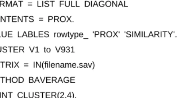
Basic objective in cluster analysis is to discover natural groupings of items or vari- ables. In general, clustering is conducted based on some similarity (or dissimilarity) matrix or the original input text data. Various measures of similarities (or dissimi- larities) between objects (or variables) are developed. We introduce a real application problem of clustering procedure in SPSS when the distance matrix of the objects (or variables) is only given as an input data. It will be very helpful for the cluster analysis of huge data set which leads the size of the proximity matrix greater than 1000, par- ticularly. Syntax command for matrix input data in SPSS for clustering is given with numerical examples.

Keywords: Clustering, dendrogram, distance matrix, syntax command.

1. Introduction

Cluster analysis is a more primitive technique in that no assumptions are made concerning the number of groups or the group structure. Grouping is done on the basis of similarities or dissimilarities (distances) between objects or variables. Cluster analysis is designed to detect hidden groups or clusters in a set of objects which are described by numerical, linguistic or structural data such that the members of each cluster behave similarly to each other with respect to given data and groups are hopefully well separated.

Most efforts to produce a rather simple group structure from a complex data set necessarily require a measure of closeness or similarity. Important considerations include the nature of the variables (discrete, continuous, binary) or scales of measurement (nominal, ordinal, interval, ratio) and subject matter knowledge.

There are two key steps in applying the clustering procedure. First, we need to decide on a measure of inter-object similarity. Secondly, we must specify a procedure for forming the clusters based on the chosen measure of similarity. Most efforts to produce a rather simple group structure from a complex data set necessarily require a measure of closeness or similarity. When items are clustered, proximity is usually indicated by some sort of distance.

Dillon and Goldstein (1984) have discussed another approach to cluster analysis, graphical methods.

1

Professor, School of Computer & Information Communication Engineering, Catholic University of

Daegu, Gyungbuk 712-702, Korea. E-mail: [email protected]

Modern statistical packages such as SAS, SPSS or Matlab provide various clustering algo- rithms and widely used in many areas. Cole (1999) made a SAS macro program code that implements simple nonparametric bootstrap statistical inference. Jain and Moreau (1987) considered a method estimating the number of clusters in a data set by using the bootstrap technique. Thomas and Timothy (1987) compared statistical packages SPSS, Biomed, and SAS in social sense. Cho and Kim (2008) compared statistical packages in survival analysis view point. Lee (2004) considered a clustering of microarray data. As far as cluster analysis concerned, in most statistical packages, the type of input data is text data which can be seen in worksheet. Most of statistical packages are providing clustering analysis based on the text type input data. The type of input data can be a value for each variables.

Suppose the p × p matrix type data which represent the distance or similarities between objects (or variables) is only available due to many reasons. There are many situations which we can get only p × p matrix of proximities that can be used as an input data. For example, we can not use the clustering procedure any more because the system could not calculate the required distances between objects (or variables) when the elements of some cluster changed to the other cluster. In some cases, we can not have the original data and we can get the distance matrix only. In such cases, we need a clustering procedure based on the input data of matrix type.

In this paper, we consider cluster analysis in SPSS, particularly the input matrix type of proximity data is given. Of course, SAS can handle the matrix input data type in clustering procedure. But in many cases, we can handle SPSS more simply than SAS due to the menu driven program. Clustering syntax command for matrix input data of this paper will be useful to the clustering of huge data set, particularly.

2. SPSS syntax command for matrix input data

Suppose we already have p × p matrix of proximities that can be used as input. However, when we run the cluster procedure on this data, the procedure computes a distance matrix from the data, as if the data were case-level values on the variables. How can we indicate that the data already comprises a proximity matrix?

In order to have the matrix of proximities recognized as such by the cluster procedure, we must add two variables to the matrix file and we must run the procedure as a syntax command. The two variables are ROWTYPE and VARNAME . Both variables are string variables with a width of 8 characters.

The variable ROWTYPE must be the first variable in the file. It will typically have the value “PROX” in all p rows. Correlations are sometimes used as similarity measures in cluster analysis. If the proximity matrix is a correlation matrix, then ROWTYPE will have the value “CORR” in all p rows of the data file. When the values of ROWTYPE equal

“PROX”, the cluster procedure will treat the matrix vlaues as distances by default. If the matrix values are actually similarities, we need to indicate this by assigning a value label of “SIMILARITY” to the ROWTYPE value “PROX”. For a matrix of distance values, we can assign “PROX” a value label of “DISSIMILARITY”, but this is not necessary.

The variable VARNAME must be the second variable in the file. A symmetric proximity

matrix assumed by the cluster, with row p and column p referring the same object. Each

column of the matrix will have a variable name associated with it. The value of VARNAME

in each row of the file will be the variable name associated with that row’s object, that is, the variable name for the corresponding column.

Once the new variables have been added to the matrix file, we can run the cluster analysis from a syntax window with the CLUSTER command. CLUSTER command must include the subcommand. The desired command is as follows.

MATRIX DATA VARIABLES = V1 to V931 /FORMAT = LIST FULL DIAGONAL /CONTENTS = PROX.

VALUE LABLES rowtype_ 'PROX' 'SIMILARITY'.

CLUSTER V1 to V931 /MATRIX = IN(filename.sav) /METHOD BAVERAGE /PRINT CLUSTER(2,4).

Figure 2.1 Syntax command of clustering for matrix input data.

The first line command of Figure 2.1 means that we will handle matrix type data which is consist of 931 variables with the variable name V1 through V931. The second line in Figure 2.1 means the format type of input matrix. The third line should be specified. When the correlation matrix is used, “PROX” should be changed to “CORR”. The 4th line also should be specified for the similarity matrix. The value of rowtype in the data will indicate a matrix of proximities. The 5th line in Figure 2.1 is the key line in cluster procedures. We should note the variable name in the input file and the variable name of the command line should be the same ones. The 6th line command in Figure 2.1 specifies the input matrix data file. The 7th line selects the linkage method such as single, complete, ward and so on.

The final line request a table of the cluster membership of each case for the two, three, and four cluster solutions.

3. Numerical Example

In this section, we consider artificial numerical data for clustering which is given in Johnson and Wichern (1982). The distance between 5 observations are given in Figure 3.1.

Figure 3.1 The distance between objects.

For the clustering procedure based on the distance matrix of Figure 3.1, we should pre- pare another matrix file such as Figure 3.2. This matrix will be used as an input matrix for clustering procedure. As mentioned in section 2, two variables “ROWTYPE ” and “VAR- NAME ” are added to the distance matrix.

Figure 3.2 Input matrix for SPSS

With this matrix, we should use the syntax command of SPSS in Figure 3.3 for cluster analysis.

Figure 3.3 Syntax command for matrix input data

In order to get the dendrogram, we can have another syntax command as in Figure 3.4.

Figure 3.4 Syntax command for matrix input data

The SPSS output of syntax command in Figure 3.3 is in the Table 3.1 and Table 3.2 as follows.

Table 3.1 Cluster output (소속군집)

케이스 4군집 3군집 2군집

v1 1 1 1

v2 2 1 1

v2 3 2 2

v2 4 3 2

v2 1 1 1

Table 3.2 Cluster output (군집화 일정표)

단계 결합 군집

계수 처음 나타나는 군집의 단계

다음 단계

군집1 군집2 군집1 군집2

1 1 5 11.000 0 0 2

2 1 2 9.500 1 0 4

3 3 4 9.000 0 0 4

4 1 3 5.167 2 3 0

The SPSS output of syntax command in Figure 3.4 is in Figure 3.5.

Figure 3.5 Dendrogram for matrix input data

4. Conclusions

In this paper, we consider the cluster analysis based on the matrix of proximity between

objects (or variables) in SPSS. Through the numerical example we showed that the syntax

command works well. It will be helpful for SPSS user who wants to solve the cluster analysis

based on the distance matrix between objects (or variables). It will be also applicable to

the clustering of huge data set which have more than 1000 leading dimension of proximity

matrix.

References

Cho, M. and Kim, S. (2008). Comparative study on statistical packages analyzing survival model- SAS, SPSS, STATA. Journal of Korean Data & Information Science Society, 19, 487-496.

Cole, S. R. (1999). Simple bootstrap statistical inference using the SAS system. Computer Methods and Programs in Biomedicine, 60, 79-82.

Dillon, W. R. and Goldstein, M. (1984). Multivariate analysis: Methods and applications, John Wiley &

Sons.

Jain, A. K. and Moreau, J. V. (1987). Bootstrap technique in cluster analysis. Pattern Recognition, 20, 547-568.

Johnson, R. A. and Wichern, D. W. (1982). Applied multivariate statistical analysis, Prentice Hall, Engel- wood Cliffs, New Jersey.

Lee, K. (2004). Curve clustering in microarray. Journal of Korean Data & Information Science Society, 15, 575-584.

SPSS (2004). SPSS Advanced Models 12.0.1, SPSS Inc., Chicago.

Thomas, B. and Timothy, K. (1987). Comparing statistical packages: SPSS, Biomed and SAS. The Social

Science Journal , 24, 329-336.