Nexus between Indian Economic Growth and Financial Development: A Non-Linear ARDL Approach

Print ISSN: 2288-4637 / Online ISSN 2288-4645 doi:10.13106/jafeb.2020.vol7.no6.109

1

First Author and Corresponding Author. Research Scholar, Dept.

of Humanities and Social Sciences, Indian Institute of Technology Patna, India [Postal Address: Block VI, Room no. 527, Dept. of Humanities and Social Sciences, Indian Institute of Technology Patna, Bihta, Patna-801106, India]

Email: [email protected]

2

Assistant Professor, Dept. of Humanities and Social Sciences, Indian Institute of Technology Patna, India.

Email: [email protected]

© Copyright: The Author(s)

This is an Open Access article distributed under the terms of the Creative Commons Attribution Non-Commercial License (http://Creativecommons.org/licenses/by-nc/4.0/) which permits unrestricted noncommercial use, distribution, and reproduction in any medium, provided the original work is properly cited.

Nexus between Indian Economic Growth and Financial Development:

A Non-Linear ARDL Approach

Kundan KUMAR

¹

, Rajendra Narayan PARAMANIK

²

Received: March 18, 2020 Revised: March 28, 2020 Accepted: May 01, 2020

Abstract

The study examines the nexus between financial development and economic growth in India during Q1: 1996 to Q3: 2018. This study employs time-series data of real GDP and ratio of broad money to GDP as a proxy for economic and financial development, respectively.

The data are obtained from RBI database on the Indian economy. All variables are seasonally adjusted using X12-arima technique and expressed in natural logarithm form. Non-linear Autoregressive Distributed Lag (NARDL) bound test has been used to check for co- integrating relationship of these two variables. Empirical findings suggest that, unlike in the short run, in the long run financial development does impact economic growth positively. Further, a symmetric effect of positive and negative components of financial development is found for the Indian economy, whereas the effect of control variable like exchange rate and trade openness is in consonance with common economic intuition. Exchange rate is in consonance with intuitive economic logic that a fall in exchange rate makes exports cheaper and increases the quantity of export, which improves the balance of payment and leads to a rise in aggregate demand, hence improves economic growth. This paper contributes to the existing literature on India by breaking down financial indicator into positive and negative components to examine the finance-growth relationship.

Keywords: Financial Development, Economic Growth, NARDL, India JEL Classification Code: G20; O40; C10

1. Introduction

The role of financial sector development in the process of economic growth is well documented in the literature.

Financial sector development refers to both the stock market development as well as banking sector’s growth. A well- developed financial system enhances capital formation and efficient resource allocation, which in turn triggers growth.

Financial intermediaries are necessary for technological

transformation and economic growth, and development as its service monitors managers, mobilizes savings, manages risks and facilitates transactions (Schumpeter, 1911).

The financial market helps in reducing cost of borrowing money and that help firms to propel their business (Rajan

& Zingales, 1998). Most of the literature indicates that financial development is the main driver of economic growth; however the issue is unresolved because many economists hold a belief that finance is not an important factor for economic development.

There are mainly two hypotheses, first is the ‘demand- pull’ view, which emphasizes that higher economic growth leads to increase in the demand for financial services and hence foster financial market development (Adu, Marbuah,

& Mensah, 2013; Adusei & Nkrumah, 2013). Second is the

‘supply-leading’ view that suggests that economic growth follows financial development (Giri & Mohapatra, 2012; Jalil

& Feridun, 2011; Kargbo & Adamu, 2009; King & Levine,

1993; Rajan & Zingles, 1998). A well-developed financial

market streamlines financial resources to productive purposes

and promotes growth. Some author’s findings suggest there

is a bidirectional relationship between economic growth and

finance, and some argues there is no nexus between these two variables. This paper tests the interdependence between financial development and economic growth in India. The non-linear autoregressive distributed lag (NARDL) approach is applied using quarterly time-series data for time period 1996 Q1-2018 Q3. This paper contributes to the existing literature on India by breaking down financial indicators into positive and negative components to examine the finance- growth relationship.

The format of the paper is as follows. The next section briefly reviews the literature. This is followed by model specification and data description. Then follow the econometric methodology and empirical results section. The final section presents the conclusion.

2. Literature Review

The study on the nexus between financial development and economic growth has no final conclusion insofar as there are conflicting results. There are notable studies, which support the supply-leading hypothesis that economic growth follows financial development such as King and Levine (1993), Patrick (1966) and Rajan and Zingles (1998). King and Levine (1993) examined how higher levels of financial development is positively associated with economic growth using data of more than 80 countries from 1960 to 1989.

Empirical finding suggests that factors like the size of the formal sector in finance, percentage of credit to private firms, etc. are strongly related with growth and hence improve capital efficiency and its accumulation. Rajan and Zingles (1998) examine the influence of financial sector development on industrial growth using a total of 41 countries data on equity market capitalization, industries value added, gross fixed capital formation, GDP, producer price index (PPI), exchange rate, and index of industrial production (IIP) for the period from 1980 to 1990. Their findings suggest that financial sector development is very important for the rise of new firms because these firms are the main source of ideas and increases innovation, hence enhances growth indirectly.

Khan (2008) examined the interdependence between financial development and growth in Pakistan from 1961 to 2005 using ARDL bound test approach of co-integration. He founds that growth is a result of investment and financial development both in the short and the long run, however the impact in the long run is higher than in the short run.

Naik and Padhi (2015) investigated the influence of the stock market over economic growth for 27 emerging economies using heterogeneous panel causality test. Their result shows that the stock market significantly contributes to growth. In Ghana, the long-run growth effect of financial development for the period 1961-2010 has been investigated by Adu et al. (2013) using ARDL as a methodology. Their findings suggest that private-sector credit to the GDP ratio and the

private-sector credit to total credit ratio are positive and significant, whereas broad money supply to GDP ratio has significantly negative effect on growth. Beck and Levine (2004) examined the influence of stock market development and banks on economic growth for the period 1976-1998 using panel data of 40 countries. Their findings confirm that financial development is an important tool for growth.

For Pakistan’s economy, Jalil and Feridun (2011) investigated the impact of financial development on economic growth using ARDL Bound test for the period 1975-2008 and found positive and significant relation between them. Giri and Mohapatra (2012) support the supply-leading hypothesis in the Indian context for the time period from 1970-71 to 2008- 09. In Sierra Leone, Kargbo and Adamu (2009) investigated the interdependence between financial development and growth using ARDL approach of co-integration for the period 1970-2008. Their results support the supply-leading hypothesis and found that investment is the major medium through which financial development affects growth.

Some study like Zang and Kim (2007) support the demand-following hypothesis, which emphasizes that financial market development follows economic growth.

Adusei and Nkrumah (2013) investigated the relationship between financial development and economic growth using FMOLS and ECM techniques for the period 1971-2010 in Ghana. They found that the ratio of domestic credit to GDP and broad money supply to GDP ratio hinder economic growth; also, credit to private sector as a share of GDP has a positive, but insignificant relation with economic growth.

Financial integration enhances the economy’s productive capacity, provides efficient capital allocation, includes more investment and hence has a positive and significant impact on growth in Southeast Asia (Bong & Premaratne, 2019).

Ngoc (2020) investigated the impact of inflation and money supply in Vietnam using NARDL approach for the period 1990-2017 and found a negative and asymmetric impact of inflation on growth in long run whereas money supply has a positive impact on growth in both the short and long run.

In the Philippines, the effect of domestic credit and stock market liquidity on economic growth for the period 1995- 2018 is investigated by Camba and Camba (2020). Their findings support the belief that economic growth is affected by the development of banking sector and stock market.

Hye, Wizarat and Lau (2016) examined the impact of trade openness on economic growth in China for the period 1975- 2009 using ARDL and rolling regression and found that both in short as well as long-run trade openness is positively related with growth. There are studies, which support the bidirectional relation between financial development and economic growth too (Wood, 1993).

In this paper a recent method of time-series approach

named non-linear ARDL is used to examine the nexus between

financial development and growth in India using quarterly

data for the period 1996 to 2018 where asymmetric impact of financial development on economic growth is assessed.

1 2

1 0

3 4

0 0

5 0

0 1 2

3 4 5 0 1 1 1

2 1 3 1 4 1

n n

k k

n n

k k

n k

Yt Yt k FDt

k OPENt k EXCHt

k GEt k Yt FDt

OPENt EXCHt GEt et

= =

= =

=

∆ = + ∆ − + ∆

− + ∆ − + ∆

− + ∆ − + − + −

+ − + − + − +

∑ ∑

∑ ∑

∑

α α α

α α

α λ λ

λ λ λ

3. Model Specification and Data Description

The standard literature reviewed identified that financial development, real gross government expenditure, the level of trade openness of an economy and exchange rate are the major determinants of economic growth. Thus, we postulate the following model

0 1 2 3

4

µ

t t t t

t t

Y FD OPEN GE

EXCH

β β β β

β

= + + +

+ + (1)

Here Y is real output (represented by log of real GDP at market price); FD denotes financial development (proxied by ratio of broad money to GDP); trade openness is denoted by OPEN (proxied by sum of export and import to GDP ratio); GE denotes the real gross government expenditure (represented by government final consumption expenditure to GDP ratio); EXCH denotes the real exchange rate and µ is an error term. There is no lagged variable in model (1), such a model is called long run model and estimates of the coefficient β

_1,

β

_2,

β

₃

and β

₄

reflects the long run effects of exogenous variable on real output. OLS estimates of such a model could be spurious due to unit roots.

This paper is based on quarterly data covering the time period 1996Q1 to 2018Q3. All variables are seasonally adjusted using X-12-arima technique and in natural logarithm except FD and GE. The data are obtained from the database on Indian economy of RBI.

4. Econometric Methodology and Empirical Results

In addition to the long-run effects, short-run effects can be investigated through an error-correction model.

1 2

1 0

3 4

0 0

5 0

0 1 2

3 4

5 1

n n

k k

n n

k k

n k t

Yt Yt k FDt

k OPENt k EXCHt

k GEt k Et e

α α α

α α

α λ

= =

= =

=

∆ = + ∆ − + ∆

− + ∆ − + ∆

− + ∆ − + − +

∑ ∑

∑ ∑

∑

(2)

Coefficients attached to first differenced variable of OLS estimates of equation (2) reflect the short run effects.

A negative and significant value of λ measures the speed of adjustment with which the variable adjusts to their long-run equilibrium values. Since all variables are not of the same order of integration, so instead of using Engle- Granger (1987) methods, we will use bounds test of co integration and ARDL approach proposed by Pesaran, Shin and Smith (2001). By replacing E

_t-1

in equation (2) with linear combination of lagged level of variables, we can write equation (2) in the following way-

1 2

1 0

3 4

0 0

5 0

0 1 2

3 4

5 0 1 1 1

2 1 3 1 4 1

n n

k k

n n

k k

n k

Yt Yt k FDt

k OPENt k EXCHt

k GEt k Yt FDt

OPEN EXCHt GEt et

α α α

α α

α λ λ

λ λ λ

= =

= =

=

∆ = + ∆ − + ∆

− + ∆ − + ∆

− + ∆ − + − + −

+ − + − + − +

∑ ∑

∑ ∑

∑

(3(

We must establish co-integration for the long-run coefficient to be valid by applying standard F-test for joint significance of lagged level variables proposed by Pesaran et al. (2001). They produced a lower critical bound value and upper critical bound value by assuming all variable to be I(0) and I(1) respectively. If some variables are combination of level stationary and first difference stationary then upper critical bound value can also be used. We decompose the movement of the financial development indicator (FD) into its negative and positive partial sums.

FD_P = ∑

^tj₌₁

∆ FDj

⁺

= ∑

^tj₌₁

max( ∆ FDj ,0) (4) FD_N = ∑

^tj₌₁

∆ FDj

⁻

= ∑

^tj₌₁

min( ∆ FDj ,0) (5) We created DFD, first difference variable of FD then generated a series for the DFD which is positive and another series which is negative. By multiplying positive and negative series by the first difference we calculated the cumulative sum of each. The resulting sums are partial sum of positive and negative changes in broad money to GDP ratio, which we denoted by FD_P and FD_N, respectively. Using these variables we can write equation 3 in the following way.

1 2

1 0

3 4

0 0

5 6

0 0

1 1

0 1' 2

3 4

5 6

0 1 1 2 3

1 4 1 5 1

n n

k k P

n n

k N k

n n

k k

Pt Nt

Yt Yt k FD t

k FD t k OPENt

k EXCHt k GEt

k Yt FD FD OPENt

EXCHt GEt t

α α α

α α

α α

λ λ λ λ

λ λ ξ

= =

= =

= =

− −

∆ = + ∆ − + ∆

− + ∆ − + ∆

− + ∆ − + ∆

− + − + +

+

′ ′

′ ′

′

−

′ +

− + − +

∑ ∑

∑ ∑

∑ ∑

(6)

The above equation is a nonlinear autoregressive distributed lag model in which nonlinearity is addressed by creating partial sum components FD_P and FD_N. The estimate of nonlinear ARDL model (6) is shown in Table 2.

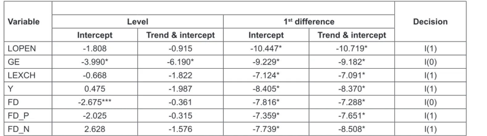
Table 1 shows the result of unit root test, which suggests that gross fixed capital expenditure to gross domestic product ratio (represented as GE) and the ratio of broad money to GDP (FD) are stationary both at the level and at their first difference, while partial sum of positive (FD_P) and negative (FD_N) changes in financial development indicator, log of exchange rate and log of ratio of sum of

export and import to GDP and log of GDP at market prices are statistically insignificant at their level and significant at their first difference. This means that there is a combination of I (0) and I (1) series. Thus, NARDL will be an appropriate estimation technique.

To test the long-run relationship an ARDL co-integration procedure is implemented. ARDL (1,1,1,0,0,1) model has been selected on the basis of akaike information criterion (AIC). The estimated result of model (1) is presented in Table 2. We can see from Table 2 that all the coefficients are statistically significant except trade openness and Table 1: Results of the Unit Root Test

Variable Level 1

^st

difference Decision

Intercept Trend & intercept Intercept Trend & intercept

LOPEN -1.808 -0.915 -10.447* -10.719* I(1)

GE -3.990* -6.190* -9.229* -9.182* I(0)

LEXCH -0.668 -1.822 -7.124* -7.091* I(1)

Y 0.475 -1.987 -8.405* -8.370* I(1)

FD -2.675*** -0.361 -7.816* -7.288* I(0)

FD_P -2.025 -0.315 -7.359* -7.651* I(1)

FD_N 2.628 -1.576 -7.739* -8.508* I(1)

Notes: * Rejection of null hypothesis at 1% level. ** Rejection of null hypothesis at 5% level. *** Rejection of null hypothesis at 10% level.

Table 2: Long-run results

Variable Coefficient Std. Error t-Statistic Prob.

Y(-1) 1.017534 0.015230 66.81134 0.0000

FD_P -0.089491 0.007786 -11.49373 0.0000

FD_P(-1) 0.087281 0.007492 11.65022 0.0000

FD_N -0.088096 0.015655 -5.627500 0.0000

FD_N(-1) 0.097113 0.016612 5.846029 0.0000

LOPEN 0.010735 0.007270 1.476542 0.1438

LEXCH -0.038402 0.010418 -3.686172 0.0004

GE -0.034863 0.069579 -0.501051 0.6177

GE(-1) 0.104242 0.071065 1.466841 0.1464

C 0.039570 0.119393 0.331423 0.7412

R-squared 0.999944

Adjusted R-squared 0.999938

S.E of regression 0.006389

Sum squared resid 0.003225

Log likelihood 328.7490

F-statistic 157188.9

Prob(F-statistic) 0.000000

Mean dependent var 9.444077

S.D. dependent var 0.810114

Akaike info criterion -7.162899

Schwarz criterion -6.883277

Hannan-Quinn criter -7.050192

Durbin-Watson stat 1.535723

*Note: p-values and any subsequent tests do not account for model selection

government expenditure. The result suggests that positive and negative components of financial development indicator and exchange rate are main factors, which are contributing to economic growth in India.

Following Oskooee (2015) proposed technique to calculate the long-run coefficient of positive and negative components of financial development indicator, negative of each coefficient is divided by the coefficient of dependent variable’s first lag, i.e. log of GDP. So, the long-run coefficient of positive component of financial development indicator is 0.087948 {– (-0.089491) / 1.017534} and long-run coefficient of negative component is 0.086577 {-(-0.088096) /1.017534}.

That is a 1 percent point increase in financial development indicator leads to 0.09 percent point increase in economic growth and 1 percent point decrease in financial development indicator leads to 0.09 almost the same decrease in economic growth. So, the instantaneous impact of positive and negative components of financial indicator is positive. The coefficients of positive and negative components are numerically close, which suggests the effect of these two variables on economic growth is symmetric.

Similarly after a lag of one period, long-run coefficient of positive (-0.087281/1.017534 = -0.085776) and negative components (-0.097113/1.017534 = -0.095439) of financial development indicator can be calculated and it is found that the effect of positive and negative components after a lag of one period is negative and their effect on growth is symmetric.

It implies that liberalization policy instantaneously increases, but after a period it diminishes the growth. It means financial liberalization can enhance the economic growth up to a certain threshold level, and further liberalization can hurt the growth (Law & Singh, 2014). The types of credit by financial system are one of the plausible reasons for this non-linear relation as Hung (2009) explains that investment

credit can promote economic growth, whereas, consumption credit may impede it.

The coefficient of exchange rate is positive {-(-0.038402)/

1.017534 = 0.037740} and statistically significant and implies that depreciation in it will enhance the growth. This result is in consonance with intuitive economic logic that a fall in exchange rate makes exports cheaper and increases the quantity of export, which improves the balance of payment and leads to a rise in aggregate demand, hence improves economic growth. This result supports the findings of Rodrik (2008) that in India GDP per capita climbed from 1 percent to 4 percent while real exchange rate was undervalued to 60 percent for the period of 1950-2000. The coefficients of government expenditure and trade openness are statistically insignificant in the long run. Table 3 presents the outcome of ARDL long-run form and Bound Test.

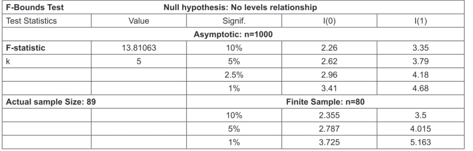
The result for bound test for co-integration suggests that there exists co-integration among variables as calculated F statistics (13.81) lies outside the upper bound I(1) (3.35).

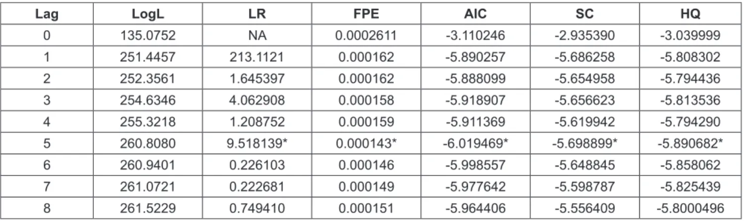
The order of lags on the first differenced variable is selected by means of the AIC and it is reported below (see Table 4).

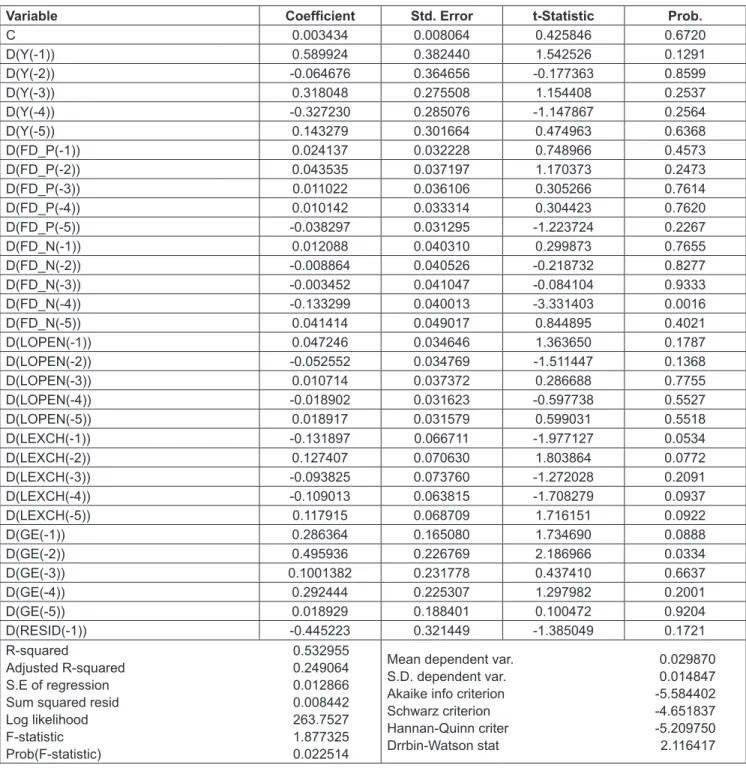
Short-run dynamics is examined through the estimation of error correction model (ECM) and Table 5 shows the results. The coefficient of error correction term is negative and it signifies convergence towards the long run equilibrium.

Table 5 shows that the coefficient of negative component of financial indicator at fourth lag is statistically significant and negative. Exchange rate is statistically significant at lags like first, second, fourth and fifth and it has negative impact at first and fourth lags but positive impact on growth at second and fifth lags in short run. Government expenditure at first two lags is found to be statistically significant and in short run it has positive impact on growth. Table 6 represents the diagnostic statistics.

Table 3: ARDL bound test of co-integration

F-Bounds Test Null hypothesis: No levels relationship

Test Statistics Value Signif. I(0) I(1)

Asymptotic: n=1000

F-statistic 13.81063 10% 2.26 3.35

k 5 5% 2.62 3.79

2.5% 2.96 4.18

1% 3.41 4.68

Actual sample Size: 89 Finite Sample: n=80

10% 2.355 3.5

5% 2.787 4.015

1% 3.725 5.163

Table 4: Statistics for lag order selection

Lag LogL LR FPE AIC SC HQ

0 135.0752 NA 0.0002611 -3.110246 -2.935390 -3.039999

1 251.4457 213.1121 0.000162 -5.890257 -5.686258 -5.808302

2 252.3561 1.645397 0.000162 -5.888099 -5.654958 -5.794436

3 254.6346 4.062908 0.000158 -5.918907 -5.656623 -5.813536

4 255.3218 1.208752 0.000159 -5.911369 -5.619942 -5.794290

5 260.8080 9.518139* 0.000143* -6.019469* -5.698899* -5.890682*

6 260.9401 0.226103 0.000146 -5.998557 -5.648845 -5.858062

7 261.0721 0.222681 0.000149 -5.977642 -5.598787 -5.825439

8 261.5229 0.749410 0.000151 -5.964406 -5.556409 -5.8000496

*indicates lag order selected by the criterion LR: sequential modified LR test statistic FPE: Final prediction error

AIC: Akaike information criterion SC: Schwarz information criterion HQ: Hannan-Quinn information criterion

Lagrange Multiplier (LM) test is employed to check the autocorrelation problem, which follows χ

²

distribution with two degrees of freedom. Observed R-square and corresponding p-value are given in the table, and they suggest to accept the null hypothesis of no serial autocorrelation in the given model. The p-value of Ramsey RESET test is greater than critical value at 5% level of significance, which rules out model misspecification and possible non-linearity.

Further to test the stability of the estimated model CUSUM and CUSUMSQ test have been performed. Figure 1 is the result of CUSUM and CUSUMSQ stability tests. Figure 1 shows that CUSUM and CUSUMSQ lies within the critical

bounds means entire coefficients are stable in the error correction model (ECM).

5. Conclusion

The relationship between financial sector development and economic growth in India has been examined over the period first quarter, 1996 to third quarter, 2018 using the bound test approach of co-integration. We found that the instantaneous impact of positive and negative components of financial indicator is positive and significant, but after a lag of one period it is negative and significant. It implies

-30 -20 -10 0 10 20 30

06 07 08 09 10 11 12 13 14 15 16 17 18

CUSUM 5% Significance

-0.2 0.0 0.2 0.4 0.6 0.8 1.0 1.2 1.4

06 07 08 09 10 11 12 13 14 15 16 17 18

CUSUM of Squares 5% Significance

Figure 1. Cumulative Sum of Recursive Residuals (CUSUM) and Cumulative Sum of Squares of

Recursive Residuals (CUSUMSQ)

Table 5: Results of ECM

Variable Coefficient Std. Error t-Statistic Prob.

C 0.003434 0.008064 0.425846 0.6720

D(Y(-1)) 0.589924 0.382440 1.542526 0.1291

D(Y(-2)) -0.064676 0.364656 -0.177363 0.8599

D(Y(-3)) 0.318048 0.275508 1.154408 0.2537

D(Y(-4)) -0.327230 0.285076 -1.147867 0.2564

D(Y(-5)) 0.143279 0.301664 0.474963 0.6368

D(FD_P(-1)) 0.024137 0.032228 0.748966 0.4573

D(FD_P(-2)) 0.043535 0.037197 1.170373 0.2473

D(FD_P(-3)) 0.011022 0.036106 0.305266 0.7614

D(FD_P(-4)) 0.010142 0.033314 0.304423 0.7620

D(FD_P(-5)) -0.038297 0.031295 -1.223724 0.2267

D(FD_N(-1)) 0.012088 0.040310 0.299873 0.7655

D(FD_N(-2)) -0.008864 0.040526 -0.218732 0.8277

D(FD_N(-3)) -0.003452 0.041047 -0.084104 0.9333

D(FD_N(-4)) -0.133299 0.040013 -3.331403 0.0016

D(FD_N(-5)) 0.041414 0.049017 0.844895 0.4021

D(LOPEN(-1)) 0.047246 0.034646 1.363650 0.1787

D(LOPEN(-2)) -0.052552 0.034769 -1.511447 0.1368

D(LOPEN(-3)) 0.010714 0.037372 0.286688 0.7755

D(LOPEN(-4)) -0.018902 0.031623 -0.597738 0.5527

D(LOPEN(-5)) 0.018917 0.031579 0.599031 0.5518

D(LEXCH(-1)) -0.131897 0.066711 -1.977127 0.0534

D(LEXCH(-2)) 0.127407 0.070630 1.803864 0.0772

D(LEXCH(-3)) -0.093825 0.073760 -1.272028 0.2091

D(LEXCH(-4)) -0.109013 0.063815 -1.708279 0.0937

D(LEXCH(-5)) 0.117915 0.068709 1.716151 0.0922

D(GE(-1)) 0.286364 0.165080 1.734690 0.0888

D(GE(-2)) 0.495936 0.226769 2.186966 0.0334

D(GE(-3)) 0.1001382 0.231778 0.437410 0.6637

D(GE(-4)) 0.292444 0.225307 1.297982 0.2001

D(GE(-5)) 0.018929 0.188401 0.100472 0.9204

D(RESID(-1)) -0.445223 0.321449 -1.385049 0.1721

R-squared 0.532955

Adjusted R-squared 0.249064

S.E of regression 0.012866

Sum squared resid 0.008442

Log likelihood 263.7527

F-statistic 1.877325

Prob(F-statistic) 0.022514

Mean dependent var. 0.029870

S.D. dependent var. 0.014847

Akaike info criterion -5.584402

Schwarz criterion -4.651837

Hannan-Quinn criter -5.209750

Drrbin-Watson stat 2.116417

Table 6: Diagnostic statistics

LM RESET CUSM CUSMS2

Obs. R-squared Prob.Chi-Square(2) Coefficient of fitted^2 P-value

S S

3.950193 0.1387 -20658163 0.8160

that financial liberalization instantaneously increases growth for a short period, but it diminishes the economic growth afterwards. We found a symmetric effect of positive and negative components on economic growth. Negative coefficient of exchange rate implies that if exchange rate increases it will harm economic growth. Stable relationship between financial sector development and growth is suggested by the plot CUSUM and CUSUMSQ test.

Financial sector development is an important ingredient for Indian economic growth. The findings of this study support the supply-lead hypothesis and suggest that government should focus not only on financial sector development, but more on other macroeconomic policies along with a stable exchange rate.

References

Adu, G., Marbuah, G., & Mensah, J. T. (2013). Financial development and economic growth in Ghana: Does the measure of financial development matter? Review of Development finance, 3(4), 192-203.

Adusei, M. (2013). Financial development and economic growth:

Evidence from Ghana. The International Journal of Business and Finance Research, 7(5), 61-76.

Beck, T., & Levine, R. (2004). Stock markets, banks, and growth:

Panel evidence. Journal of Banking & Finance, 28(3), 423-442.

Bong, A., & Premaratne, G. (2019). The Impact of Financial Integration on Economic Growth in Southeast Asia. Journal of Asian Finance, Economics and Business, 6(1), 107-119. http://

doi.org/10.13106/jafeb.2019.vol6.no1.107

Camba, A. C., & Camba, A. L. (2020). The Dynamic Relationship of Domestic Credit and Stock Market Liquidity on the Economic Growth of the Philippines. Journal of Asian Finance, Economics and Business, 7(1), 37-46. https://doi.org/10.13106/

jafeb.2020.vol7.no1.37

Engle, R. F., & Granger, C. W. (1987). Co-integration and error correction: Representation, Estimation, and Testing. Econometrica: Journal of the Econometric Society, 55(2), 251-276.

Giri, A. K., & Mohapatra, G. (2012). Financial development and economic growth: Evidence from Indian economy. International Journal of Applied Research & Studies, 1(2), 1-17.

Hung, F. S. (2009). Explaining the nonlinear effects of financial development on economic growth. Journal of Economics, 97(1), 41-65.

Hye, Q. M. A., Wizarat, S., & Lau, W. Y. (2016). The Impact of Trade Openness on Economic Growth in China: An Empirical

Analysis. Journal of Asian Finance, Economics and Business, 3(3), 27-37. https://doi.org/10.13106/jafeb.2016.vol3.no3.27.

Jalil, A., & Feridun, M. (2011). Impact of financial development on economic growth: empirical evidence from Pakistan. Journal of the Asia Pacific Economy, 16(1), 71-80.

Kargbo, S. M., Adamu, P. A., (2009). Financial development and economic growth in Sierra Leone. Journal of Monetary and Economic Integration, 9(2), 30-61.

Khan, M. A. (2008). Financial development and economic growth in Pakistan: evidence based on autoregressive distributed lag (ARDL) approach. South Asia Economic Journal, 9(2), 375- 391.

King, R. G., & Levine, R. (1993). Finance and growth: Schumpeter might be right. The Quarterly Journal of Economics, 108(3), 717-737.

Law, S. H., & Singh, N. (2014). Does too much finance harm economic growth? Journal of Banking & Finance, 41, 36-44.

Naik, P. K., & Padhi, P. (2015). On the linkage between stock market development and economic growth in emerging market economies: Dynamic panel evidence. Review of Accounting and Finance, 14(4), 363-381.

Ngoc, B. H. (2020). The Asymmetric Effect of Inflation on Economic Growth in Vietnam: Evidence by Nonlinear ARDL Approach.

Journal of Asian Finance, Economics and Business, 7(2), 143- 149. https://doi.org/10.13106/jafeb.2020.vol7.no2.143

Oskooee, M. B., & Fariditavana, H. (2015). Nonlinear ARDL approach, asymmetric effects and the J-curve. Journal of Economic Studies, 42(3), 519-530.

Patrick, H. T. (1966). Financial development and economic growth in underdeveloped countries. Economic development and Cultural change, 14(2), 174-189.

Pesaran, M. H., Shin, Y., & Smith, R. J. (2001). Bounds testing approaches to the analysis of level relationships. Journal of Applied Econometrics, 16(3), 289-326.

Rajan, R., & Zingales, L. (1998). Financial development and growth. American Economic Review, 88(3), 559-586.

Rodrik, D. (2008). The real exchange rate and economic growth. Brookings papers on economic activity, 2008(2), 365- 412.

Schumpeter, J. A., (1911). The theory of economic development, Cambridge, MA: Harvard University Press.

Wood, A. (1993). Financial development and economic growth in Barbados: Causal evidence. Savings and Development, 17(4), 379-390.

Zang, H., & Kim, Y. C. (2007). Does financial development

precede growth? Robinson and Lucas might be right. Applied

Economics Letters, 14(1), 15-19.