1. Introduction
Wind vector measurements from space have provided us with an opportunity to understand oceanographic phenomena and their scientific processes. Wind fields over ocean have been obtained from scatterometer since early 1990’s. The scatterometer winds have contributed to a variety of researches and applications, especially for climate
changes and environmental changes. However, its low spatial resolution of about 25 km limits its applicability, especially at coastal regions.
Accordingly, it makes difficulty to observe small- scale phenomena related to local air-sea interaction.
Synthetic Aperture Radar (SAR) is capable of high-resolution imaging, so that the detailed distribution of wind vectors, which is hard to be obtained from scatterometers, can be retrieved even
Estimation of Polarization Ratio for Sea Surface Wind Retrieval from SIR-C SAR Data
Tae-Sung Kim* and Kyung-Ae Park**†
*Department of Science Education, Seoul National University
**Department of Earth Science Education / Research Institute of Oceanography, Seoul National University
Abstract :Wind speeds have long been estimated from C-band VV-polarized SAR data by using the CMOD algorithms such as CMOD4, CMOD5, and CMOD_IFR2. Some SAR data with HH-polarization without any observations in VV-polarization mode should be converted to VV-polarized value in order to use the previous algorithms based on VV-polarized observation. To satisfy the necessity of polarization ratio (PR) for the conversion, we retrieved the conversion parameter from full-polarized SIR-C SAR image off the east coast of Korea. The polarization ratio for SIR-C SAR data was estimated to 0.47. To assess the accuracy of the polarization ratio coefficient, pseudo VV-polarized normalized radar cross section (NRCS) values were calculated and compared with the original VV-polarized ones. As a result, the estimated psudo values showed a good agreement with the original VV-polarized data with an root mean square error by 0.99 dB. We applied the psudo NRCS to the estimation of wind speeds based on the CMOD wind models.
Comparison of the retrieved wind field with the ECMWF and NCEP/NCAR reanalysis wind data showed relatively small rms errors of 1.88 and 1.91 m/s, respectively. SIR-C HH-polarized SAR wind retrievals met the requirement of the scatterometer winds in overall. However, the polarization ratio coefficient revealed dependence on NRCS value, wind speed, and incident angle.
Key Words :Sea Surface Wind, SAR, SIR-C, Polarization Ratio, CMOD
Received Octorber 23, 2011; Revised November 1, 2011; Accepted November 2, 2011.
†Corresponding Author: Kyung-Ae Park ([email protected])
for the coastal regions. In addition, it offers a capacity of all-weather imaging for the ocean surface irrespective of atmospheric condition, except for extreme events related to heavy rainfall. These unique imaging availabilities of SAR make it possible to observe various oceanic features such as waves (Beal et al., 1986; Dobson and Vachon, 1994; Kim, 1999), currents (Lyzenga and Marmorino, 1998; Romeiser et al., 2002; Kang and Lee, 2007), internal waves (Gasparovic et al., 1988; da Silva et al., 1997) and near-coastal and finer-scale wind fields to investigate the spatial variability of wind field (Kerbaol et al., 1998; Vandemark et al., 1998; Lehner et al., 2000;
Friedman et al., 2001; Kim, 2009). SAR-derived wind fields are now being used in various applications such as coastal environment monitoring (Korsbakken et al., 1997; Choisnard et al., 2003;
Moon et al., 2010), assimilation of ocean circulation models (Young et al., 2000; Kawamura et al., 2002;
Zabeline et al., 2011), and mapping global wind power (Furevik and Espedal, 2002; Hasager et al., 2004; Christiansen et al., 2006).
Most of SAR winds have been retrieved from C- band data with three major wind retrieval algorithms;
CMOD4 (Stoffelen and Anderson, 1997), CMOD_IFR2 (IFREMER-CERSAT, 1999), and CMOD5 (Hersbach et al., 2007). Unfortunately, all of the C-band algorithms were developed using VV- polarized observations. Several C-band SAR satellites, such as RADARSAT-1, ENVISAT, and SIR-C, carried HH-polarized SAR without any observations from VV-polarization. The models for the VV-polarization have limited the diverse utilization of SAR imagery with other frequencies and polarization states in the estimation of wind speeds. For the further understanding of spatial and temporal variation of detailed wind distributions, we need lots of wind data to acquire a sequence of wind fields from many accessible SAR data as possible.
For the extensive utilization of the data, we need a certain model for HH-polarized data.
Since there is no robust wind retrieval model for C- band HH-polarization SAR data, the previous studies have suggested a hybrid wind retrieval method combined with polarization ratio, which is defined as HH-polarized normalized radar cross section (NRCS) over VV-polarized NRCS (HH / VV), to utilize C- band SAR data imaged at HH-polarization. This approach has attempted to convert NRCS values of HH-polarized SAR to VV NRCS values by applying the polarization ratio. Wind vectors were then derived using C-band geophysical model functions (GMFs) such as CMOD algorithms that have been validated for decades (Vachon and Dobson, 2000; Horstmann et al., 2001; Monaldo et al., 2002; Kim and Moon, 2002). The results of the hybrid wind retrieval approaches have enhanced the applicability of the polarization ratio models for HH-polarized SAR data such as RADARSAT-1 and ENVISAT ASAR imagery. The rms (root mean square) errors of wind speeds retrieved from the method were by 1.38 to 1.99 m/s, which satisfied the requirement of satellite scatterometry (Monaldo et al., 2004; Feng et al., 2004; Signell et al., 2010). For more accurate retrievals, several studies have suggested some of polarization ratio coefficients optimized for RADARSAT-1 and ENVISAT ASAR.
Spaceborne Imaging Radar C-band/X-band Synthetic Aperture Radar (SIR-C/X-SAR) operated at C-, L-, and X-bands with sensor characteristics of fully polarization (HH, HV, VH, and VV). It has a capability of providing multi-frequency and multi- polarization SAR data which could be observed simultaneously and thus appropriate for the inter- comparisons between the different frequencies and polarization states. However, none of the previous researches has attempted to propose the coefficient for HH-polarized SIR-C SAR data.
In order to estimate the polarization ratio coefficient, we utilized the full-polarized SIR-C image close to the east coast of Korea as shown in the rectangles of Fig. 1. The marine environment of the coastal seas around Korea has known to be very complicated and vary with high spatial and temporal variations. The Yellow Sea is anticipated to have significant tidal effects on surface roughness of SAR images. In light of this, we selected the eastern coast of Korea. The centers of the image A and B in Fig. 1 are located at 128.73˚E, 38.82˚N and 128.87˚E, 35.12˚N, respectively.
The objectives of this study are to estimate a coefficient of polarization ratio for SIR-C SAR data, to understand the characteristics of polarization ratios by investigating relationships between the calculated coefficients and other parameters, and to assess the accuracy of SAR-derived wind vectors retrieved by using the polarization ratio coefficient.
2. Data
1) Satellite Data
SAR images from SIR-C/X-SAR were utilized to
calculate the polarization ratio (PR) coefficient and retrieve sea surface winds. Details of SIR-C SAR images used in the estimation of polarization ratio coefficient were summarized in Table 1. We used the SIR-C images acquired during the second space shuttle SIR-C/X-SAR mission (SRL-2) in October 1994. The looking angle of the SIR-C images ranges from 26.3˚ to 44.7˚ from nadir and the spatial resolution is less than 13.3 m. The image ‘A’ on 1 October 1994 was used to derive PR coefficient and the other image 'B' with dual polarization (HH / HV) acquired at 4h 55m on 3 October 1994 was utilized for wind vector retrievals using the PR coefficient.
2) Wind Data
It is important to obtain in-situ wind measurements for the comparison with satellite-derived wind field.
However, there have been only a few oceanic buoys in the seas around Korea up to now. The buoy station nearest to the study region has been operating by Korea Meteorological Administration (KMA) since 1996. Thus, it was impossible to obtain in-situ wind data over the sea surface during the study period of 1994. Instead, we have used wind measurements from ground-based Automatic Weather Station (AWS) of KMA. The AWS is located at 129.35˚E, 35.35˚N, about 25 km far from the study area. Since the wind field on land is liable to be modified by land surface friction, land orography, and other obstacles depending on local environment, it might not be a good candidate for the comparison with the wind field over the sea surface. Thus, we used the AWS wind data for a rough comparison with a SAR- derived wind vector nearest to the station.
As the other sources of wind products, we used reanalysis wind data from ECMWF (European Center for Medium-range Weather Forecasts) and NCEP/NCAR (National Centers for Environmental Prediction / National Center for Atmospheric Fig. 1. The location of SAR images used in this study, where
SIR-C SAR observed the region A with fully- polarization and B with dual-polarization.
Research) for the assessment of the retrieved wind vectors. The reanalysis winds are near-surface winds at 10 m. The wind products from ECMWF and NCEP/NCAR have spatial resolutions of 1.5˚×1.5˚
and 1.8˚×1.9˚, respectively. Time differences between the model winds and SIR-C data were relatively small by 29 minutes for the image ‘A’ and one and half hours for the image ‘B’ as shown in Table 1.
3. Method
1) Polarization Ratio
Geophysical model functions for wind retrievals have been developed by investigating empirical relationships between NRCS, wind speed, relative wind direction, and incidence angle. Representative and operational CMOD models for C-band wind retrievals are CMOD4 by Stoffelen and Anderson (1997), CMOD_IFR2 (IFREMER-CERSAT, 1999), and CMOD5 (Hersbach et al., 2007). In spite of their robustness, these algorithms are appropriate for C- band data only with VV-polarization. There has been no empirical model function for C-band HH- polarization until now. So we developed a hybrid model consisted of polarization ratio and GMFs. The polarization ratio, PR, is given by the following;
PR = (1)
where s0HHand sVV0 are the HH- and VV-polarized NRCS, respectively. Several polarization models have been proposed in the previous researches (Thompson et al., 1998; Elfouhaily et al., 1999;
Vachon and Dobson, 2000). Thompson et al. (1998) suggested a polarization ratio model using airborne scatterometer data with the following form;
PR = (2)
where q is the incidence angle of radar beam. The result of the polarization ratio model showed a good agreement with HH-polarized NRCS for incidence angles from 20˚ to 45˚ (Unal et al., 1991). Furthermore, the polarization ratio equation can be expressed as the following;
PR = (3)
where is a an adjustable parameter. When a was set to 0.6, the model function (3) yielded HH-polarized NRCS values that were similar to those estimated by (2). Setting a to 0 results in Bragg scattering, while setting a to 1 gives Kirchoff scattering. General applications for C-band HH-polarized SAR wind retrieval have used a to 0.6, whereas some researches suggested other constant values according to SAR
(1 + a tan2q)2 (1 + 2 tan2q)2 (1.6 _ sin2q)2 (1.6 + sin2q)2
s0HH s0VV Table 1. Characteristics of SIR-C image data used in tihs study
Parameter SIR-C SAR Image
Image A Image B
Frequency (GHz) 5.298 (C-band)
Polarization state Quad-polarization(HH / HV / VH / VV ) Dual-polarization(HH / HV)
Swath width (km) 21.18 45.29
Azimuthal range (km) 106.92 50.00
Resolution (m) 12.5 × 12.5 13.3 × 5.0
Look angle (deg) 26.3˚ to 30.6˚ 33.1˚ to 44.7˚
Acquired time October 1, 1994, 05h 31m 15s (UTC) October 3, 1994, 04h 55m 08s (UTC)
Central location 128.73°E, 38.82°N 129.87°E, 35.12°N
Parameter SIR-C SAR Image
Image A Image B
data. For RADARSAT-1 SAR data, several different values from 0.4 to 1.2 have been suggested in the previous studies (Horstmann et al., 2000; Vachon and Dobson, 2000; Monaldo et al., 2002).
2) Estimation of Polarization Ratio
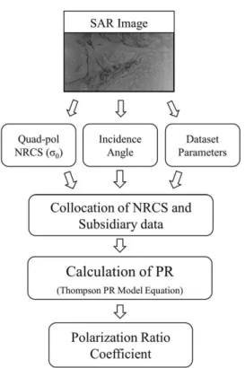
Fig. 2 indicates the schematic flow chart for the estimation of polarization ratio coefficient for SIR-C SAR data. SIR-C data were preprocessed to extract NRCS values, incidence angles, and geometric information. For SIR-C multi-look complex data with full- and dual-polarization, each pixel of digital number (DN) data has the format of 10 bytes (Quad- pol) and 6 bytes (Dual-pol), respectively. The DN values of each polarization state were decompressed to dimensionless power quantities. The calibration factor and processor gain for noise data were given by 1 and 0, respectively. The DN values were
decompressed to HH- and VV-polarizations. Then, all the extracted NRCS values and other subsidiary variables were used in the estimation of polarization ratio coefficient.
The polarization ratio has the formula in (3) and the parameter a can be solved by the following equation;
a = (4)
The calculated parameter was applied in the conversion of HH-polarized NRCS to VV-polarized NRCS. Hereafter we call it as pseudo VV-polarized NRCS. Using the pseudo VV values, we computed wind speeds and compared with the winds from original VV-polarized values.
3) Estimation of Wind Direction
SAR wind retrieval models require the information of wind directions prior to the estimation of wind speed in the CMOD algorithms. Streaks with kilometer scale generally appear on the SAR image.
Those were originated from atmospheric roll vortices or Langmuir circulation align approximately with the mean wind direction (Gerling, 1972; Leibovich, 1983;
Beal et al., 1997). This made it possible to estimate the wind direction by two-dimensional (2-D) FFT analysis on the SAR image (Wackerman et al., 1996;
Vachon and Dobson, 2000; Kim and Moon, 2002).
In case that the wind-induced streaks are not apparent on the image, the information of wind direction can be obtained from in-situ buoy measurement, scatterometer wind data, or numerical model products. Otherwise, the directions may be directly estimated from the SAR image by using 2-D Fourier transform spectrum analysis. In this study, we selected both direct and indirect methods by the FFT technique and reanalysis products. The SAR images were sampled to a small image with a window size of 10 km×10 km and then
( s0HH / sVV0 (1 + 2 tan2q) _ 1) tan2q
Fig. 2. Schematic flow chart for the estimation of polarization ratio coefficient from SIR-C SAR data.
2-D FFT was applied to obtain the directional spectra.
The direction of the spectral energy was taken as the normal to the local wind direction for that part (Kim et al., 2010). An 180˚-ambiguity problem in the determination of wind direction was solved by comparing with the reanalysis wind data.
4) Estimation of Wind Speed
Many of experimental researches have been performed to characterize the relationship between surface wind and radar backscatter for decades and produced three representative models for C-band VV- polarized SAR data as CMOD4, CMOD_IFR2, and CMOD5 algorithms. Among these, we used the most widely used CMOD4 model. The functional form of relationship between s0and wind vector is given by the followings:
s0= b0(1 + b1cos f + b3tan b2cos2f)1.6 (5)
b0= br10a+gf1(u+b) (6)
f1(y) = { (7)
where u the wind speed, f the direction of viewing relative to the wind direction which is f = 0˚ when viewing upwind, and a, b, g, b1, b2, and b3 are expanded as Legendre polynomials with 18 coefficients in total. We derived wind speeds from (5), (6), and (7) by using NRCS and wind direction.
4. Results
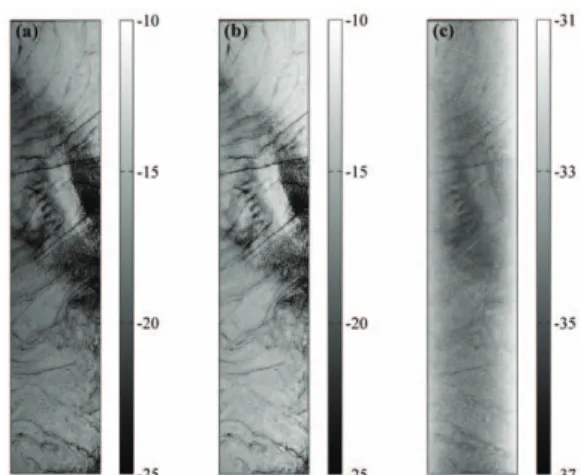
1) Difference of Polarimetric Characteristics Fig. 3 shows the distributions of SIR-C NRCS values in the polarization states of HH, VV, and HV.
VH-polarized data were not presented in Fig. 3 because cross-polarized (HV and VH) data were
regarded to be equal by the data process of Jet Propulsion Laboratory (JPL). The images show diverse features such as small-scale eddy-like patterns, slicks, and other features, which may be related to oceanic processes or oceanic-atmospheric interactions. Out of the three images, the cross- polarized data (Fig. 3c) revealed significant differences from HH or VV NRCS data (Figs. 3a and 3b). The mean values of NRCSs for the three images were -18.37 dB (HH), -15.93 dB (VV), and - 33.08 dB (HV), respectively. HV NRCS values were about twice as small as HH and VV values. The standard deviations of HH and VV NRCS were similar to 3.82 dB (HH), 3.71 dB (VV), respectively.
The cross-polarized NRCS, however, presented relatively high spatial uniformity by showing a standard deviation of 2.01 dB.
The general patterns of spatial distribution of co- polarized (HH and VV) NRCS data presented good agreement with each other, however, the magnitude of those values differed considerably. HH-polarized NRCS had smaller values than VV-polarized NRCS on the whole and the differences tended to increase as the NRCS values decreased.
_10 y 10
_10
log y 10_10< y 5 y/3.2 y > 5
Fig. 3. Images of SIR-C normalized radar cross section (s0) values (dB) acquired by (a) HH-polarization, (b) VV- polarization, and (c) HV-polarization. The SIR-C image was taken at 5h 31m on 1 October, 1994.
2) Estimation of Polarization Ratio Coefficient and Pseudo NRCS
When only HH-polarized data are available, a conversion process should be necessarily performed to generate VV-polarized data in order to use any of the CMOD wind models. Fig. 4 presents the distribution of the estimated polarization ratio values and a values at each pixel. The polarization ratio had a spatial average of 0.52 and showed no drastic spatial variability with a relatively small range from 0.49 to 0.57 (Fig. 4a).
By contrast, the parameter a indicated relatively high spatial variations from 0.31 to 0.55 with quite small frequencies in the negative values. The polarization ratio coefficient tended to increase as incidence angle increases from the right side to the left side on Fig. 4b. The spatial average of the coefficients was estimated to about 0.47. This value was quite a similar to the value suggested by Thomson et al. (1998). For the following procedure, the newly-derived mean value was used in the wind retrieval of HH-polarized SAR data as the
polarization ratio constant for SIR-C SAR data.
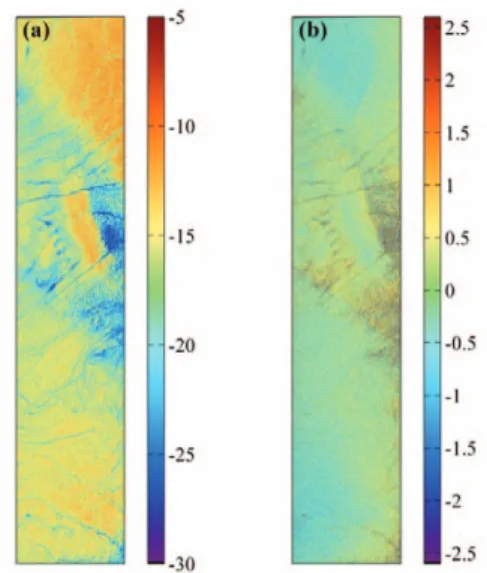
Fig. 5a shows the distributions of pseudo VV- polarized NRCS values estimated by applying the coefficient of polarization ratio to SIR-C HH- polarized data. The differences between the estimated VV-polarized values in Fig. 5a and the true NRCS values in Fig. 3b, were well matched in overall (Fig.
5b). The rms error of the NRCS differences between two data sets amounted to 0.99 dB. This implies that the estimated pseudo values were reasonaly estimated. However, it also showed some tendency that the differences were large along the low incident angles near the right side. Therefore, it is important to investigate the characteristics of the coefficients to understand the errors of wind speed retrievals.
3) Characteristics of Polarization Ratio Coefficients
In order to investigate the characteristics of polarization ratio coefficient, the a-parameter values were compared with potential error sources related to NRCS or wind speed. Fig. 6 presents the frequency Fig. 4. Spatial distributions of (a) polarization ratio values and
(b) polarization ratio coefficient values.
Fig. 5. (a) Distributions of pseudo NRCS values (dB) estimated by applying the coefficient of polarization ratio to SIR-C HH-polarized data and (b) differences between (a) and VV-polarized data (pseudo VV- polarized NRCS minus true VV-polarized NRCS).
distribution of the estimated polarization ratio coefficients with respect to a values and wind speeds retrieved from VV NRCS by using CMOD4 algorithm, where the dotted line represents the mean values of a for given wind speeds. Large standard deviations appeared at low winds. This might be related to degraded NRCS values by a low signal-to- noise ratio. The peak frequency of the most dominant
appearance was detected at a wind speed of about 3 m/s and an a value of about 0.4 (Fig. 6). This result implies that the polarization ratio coefficient is not a fixed value but a dynamic variable depending on other atmospheric and oceanic conditions.
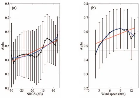
Fig. 7 illustrates the mean values of a as a function of NRCS and wind speed, where the red and blue dashed lines indicate the least-squared lines based on linear and quadratic fitting, respectively. The a values tended to increase as NRCS increased regardless of the regression methods. They were lower at ranges of less than -20 dB and higher at greater than -20 dB than the mean value of 0.47. The largest variability was detected at low NRCS around -30 dB (Fig. 7a).
The a values also revealed some dependence on wind speeds as shown in Fig. 7b. The averaged a values showed a significant positive tendency to wind speeds. As winds blew strongly, so the conversion coefficients should be increased. This implies that the dependence of the coefficient of polarization ratios on other variables including incidence angle should be
Fig. 7. Variations of a values as a function of (a) NRCS (dB) and (b) wind speed (m/s), where the red and blue dashed lines are the least-squared lines based on linear and quadratic fitting, respectively.
Fig. 6. Frequency distribution of calculated values of a as a function of wind speed, where the dashed line indicates the mean value of a at each 0.5 m/s bin of wind speeds.
considered in polarization ratio models to improve the accuracy of wind speed.
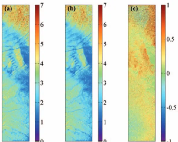
4) Application to HH-polarized SAR Data for Wind Retrieval
In order to understand differences between the wind speeds estimated from different polarized NRCS data, we compared the wind fields from VV- and HH- polarized NRCS. Fig. 8a presents the spatial distribution of the retrieved wind speeds from original VV-polarized data. The wind speeds range from 1 m/s to 7 m/s, which is quite a similar to those from the converted pseudo VV NRCS data of HH-polarized NRCS by applying the a constant (Fig. 8b). Although slightly large differences appeared for relatively strong winds (> 6 m/s) were dominant, the differences of wind speeds showed small differences in overall with an rms error of 0.37 m/s (Fig. 8c). Comparison with other wind products showed within 1.11 m/s (ECMWF) and 1.12 m/s (NCEP/NCAR), respectively.
To assess the accuracy of wind retrieval using the polarization ratio coefficient, wind field was derived from the SIR-C dual-polarized (HH and HV) image without VV-polarized observation. Fig. 9a presents the image of HH-polarized NRCS extracted from the SIR-C dual-polarized image close to the southern
coast of Korea, of which the center was located at 129.87˚E, 35.12˚N.
First of all, we calculated wind directions from the converted peudo VV-polarized NRCS by performing 2-D spectral analysis. Fig. 9b demonstrates the SIR-C SAR winds using the polarization ratio coefficient.
When compared with in-situ wind measurement from the nearest ground-based AWS, the derived wind vectors showed differences by 0.77 m/s and 58˚. The wind speed error satisfied the recommended error range of wind speeds by scatterometers. By contrast, Fig. 8. Wind speeds (m/s) from (a) original VV-polarized data and (b) converted pseudo VV-polarized data using PR ratio, and their differences between (a) and (b), (a) minus (b).
Fig. 9. (a) NRCS from C-band HH-polarized SIR-C data and (b) wind field retrieved from converted pseudo VV-polarized data.
the error of wind direction from the spectral analysis was particularly large of greater than 20˚ as general rms error of the scatterometer winds.
One of the reasons for the direction errors may come from the distance between the in-situ station and the study region, about 25 km away from the AWS. Moreover, the land orography or oceanic- atmospheric interaction might definitely modify the local wind vector on land. In addition, the error of wind direction may be caused by the existence of ocean surface modulation out of detectable range in the spectral analysis (Wackerman et al., 1996). The sub-km-scale variation of winds or low frequency modulation might induce potential error in the determination of wind direction as well. The slicks of eddy-like feature in Fig. 9a were not likely to coincide with the wind direction, but rather it might be induced by spatial changes in wind speeds and directions or by a local eddy at the sea surface without any relation to the wind field.
RMS errors between the retrieved wind speeds and reanalysis wind data sets were summarized in Table 2. Comparison of the retrieved wind vector with ECMWF and NCEP/NCAR reanalysis wind data showed rms errors by 1.88 m/s (ECMWF) and 1.91 m/s (NCEP/NCAR), which satisfied the limit of accuracy for scatterometer winds (< 2 m/s).
5. Summary and Conclusion
In this study we estimated the coefficient of
polarization ratio for HH-polarized SIR-C SAR data to convert to VV-polarized pseudo NRCS for the derivation of wind speeds in the East Sea. For the estimation of the coefficient, the a-parameter equation based on the most widely used polarization ratio model proposed by Thompson et al. (1998) was applied. The estimated polarization ratio values and a values showed somewhat opposite tendencies on the incidence angle. The polarization ratio coefficient was determined to 0.47 by taking average of each coefficient over the entire image. The estimated values of pseudo VV NRCS showed a good agreement with those of original VV NRCS dataset within an acceptable accuracy of 1 dB.
After calculating the polarization ratio coefficient, we derived wind speeds from both VV- and HH- polarized NRCS by applying the value. The retrieved wind speeds from original VV-polarized data and the derived pseudo VV NRCS showed an rms error of 0.37 m/s, which implied there was no great difference with each other. To examine the applicability of the polarization ratio coefficient in HH-polarized SAR wind retrieval, the wind field was derived from the SIR-C image that consists of HH- and HV-polarized NRCS only. Comparison with the reanalysis wind data revealed that the wind speeds from HH- polarized data were reasonably estimated with rms errors of 1.88 m/s (ECMWF) and 1.91 m/s (NCEP/NCAR). In overall, SIR-C HH-polarized SAR wind retrievals satisfied the accuracy of less than 2 m/s, which was the limit range of the scatterometer wind product.
Whereas, individual directions of wind vectors presented a considerably large rms errors of much greater than 20˚. Although the scatterometer winds have been reported to have small rms errors, each direction of the wind vectors did not always within the limit of directions. There are bunch of error sources of the scatterometer winds as well as SAR Table 2. RMS errors of wind speeds (m/s) from a quad-pol
image and a HH-pol image as compared with wind speeds from ECMWF and NCEP/NCAR datasets
SAR Image RMSE (m/s)
ECMWF NCEP/NCAR
Quad-pol image 1.11 1.12
HH-pol image 1.88 1.91
SAR Image RMSE (m/s)
ECMWF NCEP/NCAR
winds. Thus, in order to reduce the errors of SAR- derived wind vectors, a further research for estimation of the precise wind direction information should be carried out.
In addition, we analyzed the estimated values by comparing with NRCS and wind speeds to understand the characteristics of polarization ratio coefficient. The previous literature proposed that polarization ratio models were merely a function of incidence angle and a parameter. However, this study revealed that the a value depended on NRCS and wind speed as well as incidence angle. Therefore, it is suggested that a new approach should be developed to improve the accuracy of HH-polarized SAR wind retrievals by considering the NRCS dependency in polarization ratio model and derivation of the PR coefficient.
Acknowledgements
This study was supported by the Korea Aerospace Research Institute (KARI). We would like to acknowledge Korea Meteorological Administration (KMA) for providing partial support and wind measurements for this study. We are also grateful to two unknown reviewers for their helpful comments.
References
Beal, R.C., T.W. Gerling, D.E. Irvine, F.M. Monaldo, and D.G. Tilley, 1986. Spatial variations of ocean surface wave directional spectra, Journal of Geophysical Research, 91(C2):
2433-2449.
Beal, R.C., V.N. Kudryavtsev, D.R. Thompson, S.A.
Grodsky, D.G. Tilley, V.A. Dulov, and H.C.
Graber, 1997. The influence of the marine atmospheric boundary layer on ERS-1
synthetic aperture radar imagery of the Gulf Stream, Journal of Geophysical Research, 102(3): 5799-5814.
Choisnard, J., M. Bernier, and G. Lafrance, 2003.
RADARSAT-1 SAR scenes for wind power mapping in coastal area: Gulf of St-Lawrence case, International Geoscience and Remote Sensing Symposium, IGARSS’03, 4: 2700- 2702.
Christiansen, M.B., W. Koch, J. Horstmann, C.B.
Hasager, and M. Nielsen, 2006. Wind resource assessment from C-band SAR, Remote Sensing of Environment, 105(1): 68- 81.
da Silva, J.C.B., I.S. Robinson, D.R.G. Jeans, and T.
Sherwin, 1997. The application of near-real time ERS-1 SAR data for predicting the location of internal waves at sea, International Journal of Remote Sensing, 18: 3507-3517.
Dobson, F.W. and P.W. Vachon, 1994. The Grand Banks ERS-1 SAR wave spectra validation experiment: Program overview and data summary, Atmosphere-Ocean, 32(1): 7-29.
Elfouhaily, T., D. Thompson, D. Vandemark, and B.
Chapron, 1999. A new bistatic model for electromagnetic scattering from perfectly conducting random surfaces, Waves in Random Media, 9(3): 281-294.
Feng, Q., M. Fang, Y. Liu, and L. Wang, 2004. Wind retrieval over the China Seas using satellite synthetic aperture radar, International Geoscience and Remote Sensing Symposium, IGARSS’04, 5: 3169-3171.
Friedman, K.S., T.D. Sikora, W.G. Pichel, P.
Clemente-Colon, and G. Hufford, 2001.
Using spaceborne synthetic aperture radar to improve marine surface analyses, Weather Forecast, 16: 270-276.
Furevik, B.R. and H.A. Espedal, 2002. Wind energy
mapping using synthetic aperture radar, Canadian Journal of Remote Sensing, 28(2):
196-204.
Gasparovic, R.F., J.R. Apel, and E.S. Kasischke, 1988. An overview of the SAR internal wave signature experiment, Journal of Geophysical Research, 93(C10): 12304-12316.
Gerling, T.W., 1972. Structure of the surface wind field from Seasat SAR, Journal of Geophysical Research, 91(C2): 2308-2320.
Hasager, C.B., E. Dellwik, M. Nielsen, and B.
Furevik, 2004. Validation of ERS-2 SAR offshore wind-speed maps in the North Sea, International Journal of Remote Sensing, 25:
3817-3841.
Hersbach, H., A. Stoffelen, and S. de Haan, 2007. An improved C-band scatterometer ocean geophysical model function: CMOD5, Journal of Geophysical Research, 112:
C03006, doi:10.1029/2006JC003743.
Horstmann, J., W. Koch, S. Lehner, and R. Tonboe, 2000. Wind retrieval over the ocean using synthetic aperture radar with C-band HH polarization, IEEE Transactions on Geoscience and Remote Sensing, 38(5): 2122-2131.
Horstmann, J., W. Koch, S. Lehner, and R. Tonboe, 2001. Coastal high resolution wind fields retrieved from RADARSAT-1 ScanSAR, International Geoscience and Remote Sensing Symposium, IGARSS’02, 4: 1747-1749.
IFREMER-CERSAT, 1999. Off-line wind scatterometer ERS products: user manual, Technical Report C2-MUT-W-01-IF, IFREMER-CERSAT.
Kang, M.K. and H. Lee, 2007. Estimation of ocean current velocity near Incheon using Radarsat- 1 SAR and HF-radar data, Korean Journal of Remote Sensing, 23(5): 421-430.
Kawamura, H., T. Shimada, M. Shimada, A.
Kortcheva, and I. Watabe, 2002. L-band SAR wind-retrieval model function and its application for studies of coastal surface winds and wind waves, International Geoscience and Remote Sensing Symposium, IGARSS’02, 3: 1884-1886.
Kerbaol, V., B. Chapron, and P. Queffeulou, 1998.
Analysis of the wind field during the Vendee Globe race: A kinematic SAR wind speed algorithm, Earth Observation Quarterly, 59:
16-19.
Kim, D.J. and W.I. Moon, 2002. Estimation of sea surface wind vector using RADARSAT data, Remote Sensing of Environment, 80(1): 55- 64.
Kim, D.J., 2009. Wind retrieval from X-band SAR image using numerical ocean scattering model, Korean Journal of Remote Sensing, 25(3): 243-253.
Kim, T.R., 1999. Some application of SAR imagery to the coastal waters of Korea, Korean Journal of Remote Sensing, 15(1): 61-71.
Kim, T.S. K.A. Park, and W.I. Moon, 2010. Wind vector retrieval from SIR-C SAR data off the east coast of Korea, Journal of Korean Earth Science Society, 31(5): 475-487.
Korsbakken, E., J.A. Johannessen, and O.M.
Johannessen, 1997. Coastal wind field retrievals from ERS SAR images, International Geoscience and Remote Sensing Symposium, IGARSS’97, 3: 1153-1155.
Lehner, S., J. Schulz-Stellenfleth, B. Schattler, H.
Breit, and J. Horstmann, 2000. Wind and wave measurements using complex ERS-2 SAR wave mode data, IEEE Transactions on Geoscience and Remote Sensing, 38(5): 2246- 2257.
Leibovich, S., 1983. The form and dynamics of Langmuir circulations, Journal of Fluid
Mechanics, 15: 391-427.
Lyzenga, D.R. and G.O. Marmorino, 1998.
Measurement of surface currents using sequential synthetic aperture radar images of slick patterns near the edge of the Gulf Stream, Journal of Geophysical Research, 103: 18769-18777.
Monaldo, F.M., D.R. Thompson, R.C. Beal, W.G.
Pichel, and P. Clemente-Colon, 2002.
Comparison of SAR-derived wind speed with model predictions and ocean buoy measurements, IEEE Transactions on Geoscience and Remote Sensing, 39(12):
2587-2600.
Monaldo, F.M., D.R. Thompson, W.G. Pichel, and P.
Clemente-Colon, 2004. A systematic comparison of QuikSCAT and SAR ocean surface wind speeds, IEEE Transactions on Geoscience and Remote Sensing, 42(2): 283- 291.
Moon, W.M., G. Staples, D.J. Kim, S.E. Park, and K.A. Park, 2010. RADARSAT-2 and coastal applications: Surface wind, waterline, and intertidal flat roughness, Proceedings of the IEEE, 98(5): 800-815.
Romeiser, R., H. Breit, M. Eineder, and H. Runge, 2002. Demonstration of current measurements from space by along-track SAR interferometry with SRTM data, International Geoscience and Remote Sensing Symposium, IGARSS’02, 1: 158-160.
Signell, R.P., J. Chiggiato, J. Horstmann, J.D. Doyle, J. Pullen, and F. Askari, 2010. High- resolution mapping of Bora winds in the northern Adriatic Sea using synthetic aperture radar, Journal of Geophysical Research, 115:
C04020, doi: 10.1029/2009JC005524.
Stoffelen, A. and D. Anderson, 1997. Scatterometer data interpretation: Estimation and validation
of the transfer function CMOD4. Journal of Geophysical Research, 102: 5767-5780.
Thompson, D., T. Elfouhaily, and B. Chapron, 1998.
Polarization ratio for microwave backscattering from the ocean surface at low to moderate incidence angles, International Geoscience and Remote Sensing Symposium, IGARSS’98, 3: 1671-1673.
Unal, C.M.H., P. Snooji, and P.J.F. Swart, 1991. The Polarization-dependent relation between radar backscatter from the ocean surface and surface wind vectors at frequencies between 1 and 18 GHz, IEEE Transactions on Geoscience and Remote Sensing, 29(4): 621-626.
Vachon, P. and F. Dobson, 2000. Wind retrieval from RADARSAT SAR images: selection of a suitable C-band HH polarization wind retrieval model, Canadian Journal of Remote Sensing, 26(4): 306-313.
Vandemark, D., P.W. Vachon, and B. Chapron, 1998.
Assessment of ERS-1 SAR wind speed estimates using an airborne altimeter, Earth Observation Quarterly, 59: 5-8.
Wackerman, C., C. Rufenach, R. Schuchman, J.
Johannessen, and K. Davidson, 1996. Wind vector retrieval using ERS-1 synthetic aperture radar imagery, Journal of Geophysical Research, 34: 1343-1352.
Young, G.S., T.D. Sikora, and N.S. Winstead, 2000.
Inferring marine atmospheric boundary layer properties from spectral characteristics of satellite-borne SAR imagery, Monthly Weather Review, 128: 1506-1520.
Zabeline, V., L. Neil, W. Perrie, P.W. Vachon, C.
Fogarty, S.K. Khurshid, S. Komarov, and B. Zhang, 2011. RADARSAT application in ocean wind measurements, International Geoscience and Remote Sensing Symposium, IGARSS’11, 3622-3625.