Parametric Estimations for Parameter Changes in the Exponential Distribution

2005, Vol. 16, No. 1, pp. 107∼114

Parametric Estimations for Parameter Changes in the Exponential Distribution

Changsoo Lee ¹⁾ ․ Yeunggil Moon ²⁾

Abstract

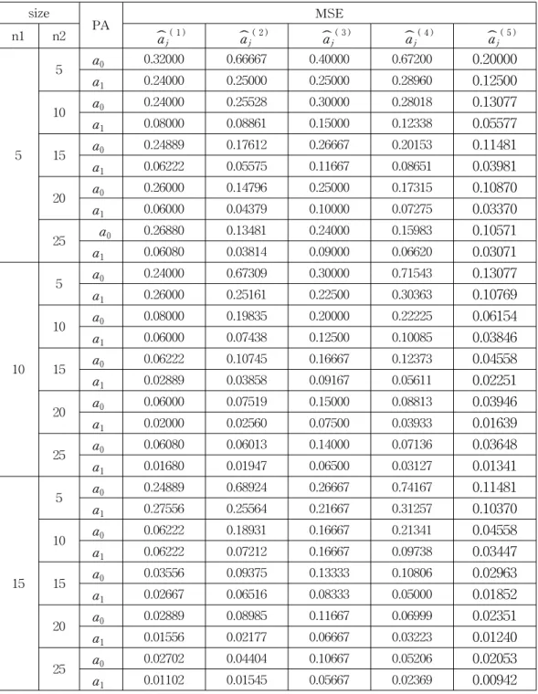
We shall consider parametric estimations for the scale parameter in the exponential distribution when the parameter is function of a known exposure level, and obtain expectations and variances for their proposed estimators. And we shall compare numerically efficiencies for proposed estimators of the scale parameter in the small sample sizes.

Keywords : Efficiency, Exponential model, MLE, Modified MLE, Unbiased estimator

1. Introduction

Many authors have utilized the exponential distribution because of its wide applicability in reliability engineering and statistical inferences (See Saunders and Mann(1985) and Bain and Engelhart(1987)). Here we shall consider parametric estimations in the exponential distribution when its scale parameter is a function of a known exposure level t, which often occurs in the engineering and physical phenomena. Woo and Yoon(1990) considered unified jackknife estimates for parameter changes in Pareto distribution. Woo and Ali(1994) studied the jackknife parametric estimations in the exponential distribution when its scale and location parameters change a function of environment dosage. And Woo and Lee(2000) studied an application of the Weibull distribution to the strength of materials when its shape and scale parameters are functions of a known exposure level. And Kim and Lee(2002) proposed several estimators for the shape and the scale parameters

1) First Author : Assistant Professor, School of Multimedia Engineering, Kyungwoon University, Kumi, 730-850, Korea.

E-mail : [email protected]

2) Assistant Professor, Department of Quality Management, Kangwon Tourism College,

Taebaek, 235-711, Korea.

in a generalized uniform distribution when both parameters are polynomials of a known exposure level and compared numerically efficiencies for several proposed estimators of the shape and scale parameters in the generalized uniform distribution.

The purpose of this work is to estimate the scale parameter in the exponential distribution when parameter changes a function of an environment dosage, say t.

In this paper, we shall propose several estimators for the scale parameter in the exponential distribution with the same location and scale parameters when the scale parameter is function of a known exposure level t , and obtain mean and variances for their proposed estimators. And we shall compare numerically efficiencies for the several proposed estimators for the scale parameter in the exponential model with the same location and scale parameters in the small sample sizes.

2. Estimations for Parameter Changes

We shall consider the exponential distribution with the p.d.f.

f ( x ;θ( t)) = { ^{θ( t) 1 e}

- x - θ( t)

θ( t) ,0 < θ( t) < x, 0 , elsewhere,

which has mean 2⋅θ( t) and variance θ(t) ² , denoted by X∼ EXP (θ(t)).

Goutis & Casella(1999) studied a normal distribution with the same mean and variance only when two location and scale parameters equal. Woo(2003) have considered jackknifing and typical point and interval estimators of parameter and right tail probability in an exponential distribution with the same location and scale parameters.

Here, we shall consider unified estimates for the parameter change of exposure levels in the exponential distribution with the same location and scale parameters when the scale parameter _{θ( t)} is functions of t ;

θ( t) = a ₀ + a ₁ t + a ₂ t ² + … + a _r t ^r , t > 0 and a i > 0, i = 0,1,…,r.

Assume _{X 1j , … ,X}

jj

are random samples taken from _X

∼ EXP (θ( t

)), j = 1,2,…r + 1 , _t

_≠t

for _i≠k and random vector X ₁ , … , X _{r + 1} are independent, And Let _{X ( 1)j , … ,X ( n}

j

) j be the corresponding order statistics for

X _1j , … ,X

.

Define the following notation :

det [ t ⁰ _i ,…,t ^r _i ] =

︳

︳

︳ ︳

︳ ︳

︳ ︳

︳ ︳

︳ ︳

︳ ︳

︳ ︳

︳

︳

︳

︳ ︳

︳ ︳

︳ ︳

︳ ︳

︳ ︳

︳ ︳

︳ ︳

︳ 1 t ₁ t ² ₁ … t ^r ₁ 1 t ₂ t ² ₂ … t ^r ₂

⋅ ⋅ ⋅ … ⋅

⋅ ⋅ ⋅ … ⋅

1 t _{r + 1} t ² _{r +1} … t ^r _{r + 1} .

By the maximum likelihood(ML) method, we can obtain the ML estimators for a _j , j = 0,1,…,r, ;

a _j

ˆ ^{( 1 )} = det [ t ⁰ _i ,…,t ^{j - 1} _i ,X _{( 1) i} ,t ^{j + 1} _i ,…,t ^r _i ] det [ t ⁰ _i ,…,t ^r _i ] . Note that

︳

︳

︳ ︳

︳ ︳

︳ ︳

︳ ︳

︳

︳

︳

︳ ︳

︳ ︳

︳ ︳

︳ ︳

︳ a ₁₁ a ₁₂ … a _1n a ₂₁ a ₂₂ … a _2n

⋅ ⋅ … ⋅ a ₁₁ a ₁₂ … a ₁₁

= a _k1 A _k1 + a _k2 A _k2 + … + a _kn A _kn , (2.1)

where A _kj = ( - 1) ^{k + j} D _kj and D _kj is minor determinant for a _kj eliminated k-row and j-column.

From (2.1), the expectations and variances of these MLE's a ˆ _j ^{( 1 )} for a _j in the exponential distribution can be obtained by

E( a ˆ _j ^{( 1 )} ) = a _j + ^{r + 1} ∑

k = 1

det [t ⁰ _i , … ,t ^{j - 1} _i ,t ^{j + 1} _i , … ,t ^r _i ] _i≠k det [t ⁰ _i , … ,t ^r _i ]

θ( t _k ) n _k and

VAR( a ˆ _j ^{( 1 )} ) = ^{r + 1} ∑

k = 1

det ² [t ⁰ _i , … ,t ^{j - 1} _i ,t ^{j + 1} _i , … ,t ^r _i ] _i≠k

det ² [t ⁰ _i , … ,t ^r _i ] ⋅ θ ² (t _k )

n ² _k , (2.2)

where det [ t ⁰ _i ,…,t ^{j - 1} _i ,t ^{j + 1} _i ,…,t ^r _i ] _i≠k is a minor determinant eliminated k-row and

( j + 1)-column in the determinant, det [ t ⁰ _i ,…,t ^r _i ].

Since MLE ˆ a _j ^{( 1 )} for a _j is biased estimator, we can propose following unbiased estimator for a j in the exponential distribution ;

a _j ˆ ^{( 2 )} =

det [ t ⁰ _i ,…,t ^{j - 1} _i , n _i

n _i +1 X _{( 1) i} ,t ^{j + 1} _i ,…,t ^r _i ] det [ t ⁰ _i ,…,t ^r _i ] .

And the variances of these unbiased estimator's a ˆ _j ^{( 2 )} for a j can be obtained by

VAR( a ˆ _j ^{( 2 )} ) = ∑

r + 1 k = 1

det ² [t ⁰ _i , … ,t ^{j - 1} _i ,t ^{j + 1} _i , … ,t ^r _i ] _i≠k

det ² [t ⁰ _i , … ,t ^r _i ] ⋅ θ ² (t _k )

( n _k +1) ² . (2.3) Also, we can propose another unbiased estimator for a j in the exponential distribution as follows ;

a _j

ˆ ^{( 3 )} = det [ t ⁰ _i ,…,t ^{j - 1} _i , X _i /2,t ^{j + 1} _i ,…,t ^r _i ] det [ t ⁰ _i ,…,t ^r _i ] ,

where X _i = 1 n _i ∑

n

k = 1 X _ki is the sample mean.

From (2.1), the variances of these unbiased estimator's a ˆ _j ^{( 3 )} for a j can be obtained by

VAR( a ˆ _j ^{( 3 )} ) = ∑

r + 1 k = 1

det ² [t ⁰ _i , … ,t ^{j - 1} _i ,t ^{j + 1} _i , … ,t ^r _i ] _i≠k

det ² [t ⁰ _i , … ,t ^r _i ] ⋅ θ ² (t _k )

4n ² _k . (2.4) Next, we can propose the modified MLE for a j in the exponential distribution as follows ;

a _j ˆ ^{( 4 )} =

det [ t ⁰ _i ,…,t ^{j - 1} _i , n _i -1

n _i X _{( 1) i} ,t ^{j + 1} _i ,…,t ^r _i ] det [ t ⁰ _i ,…,t ^r _i ] .

From (2.1), the expectations and variances of these modified MLE's a ˆ _j ^{( 4 )} for

a _j can be obtained by

E( a ˆ _j ^{( 4 )} ) = a _j + ∑

r + 1 k = 1

det [t ⁰ _i , … ,t ^{j - 1} _i ,t ^{j + 1} _i , … ,t ^r _i ] _i≠k det [t ⁰ _i , … ,t ^r _i ]

θ( t _k ) n ² _k and

VAR( a ˆ _j ^{( 4 )} ) = ^{r + 1} ∑

k = 1

det ² [t ⁰ _i , … ,t ^{j - 1} _i ,t ^{j + 1} _i , … ,t ^r _i ] _i≠k

det ² [t ⁰ _i , … ,t ^r _i ] ⋅ ( n _k -1) ²

n ⁴ _k θ ² (t _k ). (2.5)

Let θ ˆ _{U ( t j ) =} ^{n j}

n _j +1 X _{( 1 )j} and θ ˆ _M ( t _j ) = 1 2 X _j . For 0≤s≤1, θ ˆ s _{= s⋅ θ}

ˆ U ( t _j ) + ( 1 - s) ⋅ θ ˆ _M ( t _j ) is unbiased estimators for θ( t _j ) and it has minimum variance when s = n _j +1

n _j +3 ( n _j > 4) (see Woo(2003)).

Therefore, we can propose following unbiased estimators a ˆ _j ^{( 5 )} for a _j

a _j ˆ ^{( 5 )} =

det [ t ⁰ _i ,…,t ^{j - 1} _i , n _i

n _i +3 X _{( 1) i} + 1

2( n _i +3) ⋅ X _i ,t ^{j + 1} _i ,…,t ^r _i ]

det [ t ⁰ _i ,…,t ^r _i ] .

From (2.1), their variances for unbiased estimators a ˆ _j ^{( 5 )} for a _j can be obtained as

VAR( a ˆ _j ^{( 5 )} ) = ∑

r + 1 k = 1

det ² [t ⁰ _i , … ,t ^{j - 1} _i ,t ^{j + 1} _i , … ,t ^r _i ] _i≠k

det ² [t ⁰ _i , … ,t ^r _i ] ⋅ 1

n _k (n _k + 3) θ ² (t _k ). (2.6)

From the results (2.2) through (2.6), proposed estimators ^ˆ _a

^{( i )} , i = 1,2,3,4,5, are MSE consistent for a _j respectively.

From the results of expectations and variances for several proposed estimators for _a

, Table 1 shows the numerical values of mean squared errors for proposed estimators in an assumed exponential distribution for sample sizes n ₁ =5(5)25, n ₂

=5(5)25, _{a 0 = 0, a 1 = 1} , and _{t 1 = 1} , _{t 2 = 2} . From Table 1, estimator ˆ _{a 0} ^{( 5 )} is more

efficient than other proposed estimators for _{a 0} and estimator ˆ _{a 1} ^{( 5 )} is more

efficient than other proposed estimators for _{a 1} in the exponential distribution.

References

1. Kim, J.D. and Lee, J.C.(2002), Unified Estimations for Parameter Changes in a Generalized Uniform Distribution, Journal of Korean Data &

Information Science Scociety, Vol. 13(2), 295-305.

2. Bain, L.J. and Engelhart, M.(1987), Introduction to Probability and Mathematical and Statistics, PWS- KENT, Boston, U.S.A.

3. Goutis, C. and Casella, G.(1999), Explaining the Saddlepoint Approximation, The American Statistician, Vol 53(3), 216-224.

4. Saunders, S.C. and Mann, N.R.(1985), Workshop on Statistical Reliability for Engineers and cientists, National Bureau of Standard.

5. Woo, J.S.(2003), Bais Reducing Estimators in an Exponential Distribution, To Appear.

6. Woo, J.S. and Ali, M.M.(1994). Unified Jackknife Estimation for

Parameter Changes in the Exponential Distribution, Journal of Statistical Studies, Vol. 14, 20-23

7. Woo, J.S. abd Lee, C.S.(2000). Jackknife Estimates for Parameter Changes in the Weibull Distribution, The Korean Communications in Statistics, Vol 7(1), 199-209.

8. Woo, J.S. and Yoon. G.E.(1990). Unified Estimation for Parameter

Changes in a Two Pareto Distribution, Journal of Nature Sciences, Vol

9, 41-48.

Table 1. MSEs of proposed estimators for parameter changes in the exponential distribution ( _{a 0 = 0,a 1 = 1} , _{t 1 = 1} , _{t 2 = 2} )

size

PA MSE

n1 n2 ˆ a

^{( 1 )} _a

ˆ

^{( 2 )} _a

ˆ

^{( 3 )} _a

ˆ

^{( 4 )} _a

ˆ

^{( 5 )}

5

5 a 0 0.32000 0.66667 0.40000 0.67200 0.20000

a ₁ 0.24000 0.25000 0.25000 0.28960 0.12500

10 a 0 0.24000 0.25528 0.30000 0.28018 0.13077

a ₁ 0.08000 0.08861 0.15000 0.12338 0.05577

15 a 0 0.24889 0.17612 0.26667 0.20153 0.11481

a ₁ 0.06222 0.05575 0.11667 0.08651 0.03981

20 a 0 0.26000 0.14796 0.25000 0.17315 0.10870

a ₁ 0.06000 0.04379 0.10000 0.07275 0.03370

25 _{a 0} 0.26880 0.13481 0.24000 0.15983 0.10571

a 1 0.06080 0.03814 0.09000 0.06620 0.03071

10

5 a 0 0.24000 0.67309 0.30000 0.71543 0.13077

a 1 0.26000 0.25161 0.22500 0.30363 0.10769

10 a ₀ 0.08000 0.19835 0.20000 0.22225 0.06154

a 1 0.06000 0.07438 0.12500 0.10085 0.03846

15 a ₀ 0.06222 0.10745 0.16667 0.12373 0.04558

a 1 0.02889 0.03858 0.09167 0.05611 0.02251

20 a ₀ 0.06000 0.07519 0.15000 0.08813 0.03946

a 1 0.02000 0.02560 0.07500 0.03933 0.01639

25 a ₀ 0.06080 0.06013 0.14000 0.07136 0.03648

a 1 0.01680 0.01947 0.06500 0.03127 0.01341

15

5 a ₀ 0.24889 0.68924 0.26667 0.74167 0.11481

a 1 0.27556 0.25564 0.21667 0.31257 0.10370

10 a 0 0.06222 0.18931 0.16667 0.21341 0.04558

a 1 0.06222 0.07212 0.16667 0.09738 0.03447

15 a 0 0.03556 0.09375 0.13333 0.10806 0.02963

a ₁ 0.02667 0.06516 0.08333 0.05000 0.01852

20 a 0 0.02889 0.08985 0.11667 0.06999 0.02351

a ₁ 0.01556 0.02177 0.06667 0.03223 0.01240

25 a 0 0.02702 0.04404 0.10667 0.05206 0.02053

a ₁ 0.01102 0.01545 0.05667 0.02369 0.00942

size

PA

MSE

n1 n2 ˆ a

^{( 1 )} _a

ˆ

^{( 2 )} _a

ˆ

^{( 3 )} _a

ˆ

^{( 4 )} _a

ˆ

^{( 5 )}

20

5 a 0 0.26000 0.70068 0.25000 0.75769 0.10870

a 1 0.28500 0.25850 0.21250 0.31810 0.10217

10 a 0 0.06000 0.18725 0.15000 0.21165 0.03946

a ₁ 0.06500 0.07161 0.11250 0.09666 0.03294

15 a 0 0.02889 0.08920 0.11667 0.10285 0.02351

a ₁ 0.02722 0.03402 0.07917 0.04797 0.01699

20 a 0 0.02000 0.05442 0.10000 0.06354 0.01739

a ₁ 0.01500 0.02041 0.06250 0.02971 0.01087

25 a 0 0.01680 0.03821 0.09000 0.04503 0.01441

a ₁ 0.00980 0.01399 0.05250 0.02093 0.00789

25

5 a 0 0.26880 0.70874 0.24000 0.76835 0.10571

a ₁ 0.29120 0.26052 0.21000 0.32181 0.10143

10 a 0 0.06080 0.18690 0.14000 0.21157 0.03648

a 1 0.06720 0.07152 0.11000 0.09661 0.03220

15 a 0 0.02702 0.08729 0.10667 0.10068 0.02053

a 1 0.02809 0.03354 0.07667 0.04713 0.01624

20 a ₀ 0.01680 0.05197 0.00900 0.06063 0.01441

a 1 0.01520 0.01980 0.06000 0.02857 0.01012

25 a ₀ 0.01280 0.03550 0.08000 0.04176 0.01143

a 1 0.00960 0.01331 0.05000 0.01965 0.00714

[ received date : Oct. 2004, accepted date : Dec. 2004 ]