Multi-User Detection using Support Vector Machines

Multi-User Detection using Support Vector Machines

Jung-Sik Lee*, Jae-Wan Lee*, Regular Members Jae-Jeong Hwang*, Kyung-Taek Chung* Lifelong Members

ABSTRACT

In this paper, support vector machines (SVM) are applied to multi-user detector (MUD) for direct sequence (DS)-CDMA system. This work shows an analytical performance of SVM based multi-user detector with some of kernel functions, such as linear, sigmoid, and Gaussian. The basic idea in SVM based training is to select the proper number of support vectors by maximizing the margin between two different classes. In simulation studies, the performance of SVM based MUD with different kernel functions is compared in terms of the number of selected support vectors, their corresponding decision boundary, and finally the bit error rate. It was found that controlling parameter , in SVM training have an effect, in some degree, to SVM based MUD with both sigmoid and Gaussian kernel. It is shown that SVM based MUD with Gaussian kernels outperforms those with other kernels.

Key Words : Multiuser, Detector, DS-CDMA, Support Vector Machine, Neural Network

※ This paper was supported by research funds of Kunsan National University

* School of Electronics & Information Eng., Kunsan National University ({leejs,jwlee,hwang,eoe604}@kunsan.ac.kr) 논문번호：KICS2009-06-242, 접수일자：2009년 6월 4일, 최종논문접수일자: 2009년 12월 17일

Ⅰ. Introduction

Direct-sequence code division multiple access (DS-CDMA) has emerged as the preferred techniques for increasing the channel capacity through multiple access communication systems, because the whole frequency band is used all the time and bandwidth can be utilized more efficiently. In a DS-CDMA system, the objective of the receiver is to detect the transmitted information bits of one (at mobile-end) or many (at base station) users. A variety of MUD has been proposed for DS-CDMA systems. Generally, the linear minimum mean square error (MMSE) MUD is widely used, as it is computationally very simple and can readily be implemented using standard adaptive filter techniques

^[1-2]

. The conventional linear detectors, however, fail to achieve good performance when channel suffers from high levels of additive noise or highly nonlinear distortion, or when the signal-to-noise ratio is poor. The linear detector can only work

when the underlying noise-free signal classes are linearly separable with the introduction of proper channel delays, where the channel is assumed to be stationary. In reality, the mobile channels are going to be non -stationary where it is hard to determine the proper channel delay that varies with time. If proper channel delay is not introduced in linear MUD, the signal classes from the channel output states will be non-linearly separable.

In order to get around this problem, neural network technology has been considered in implementing MUD, because it has the capability of recovering the originally transmitted signals from nonlinear decision boundary cases

^[3-7]

. In fact, neural networks have received much attention from a variety of fields, especially for telecommunication systems, because of its characteristics, such as inherent parallelism, noise immunity, knowledge storage, adaptability, and pattern classification capability

^[3-9]

.

Aazhang et al.

^[3]

first reported a study of

Fig. 1. Structure of DS-CDMA System

multi-layer perceptrons (MLP) in CDMA systems,

and showed that its performance is close to that of the optimum receiver in both synchronous and asynchronous Gaussian channels. Although the simulation results proved that back-propagation learning rule outperforms the conventional one, it still leaves a lot of difficulties, such as long training time, performance sensitivity over network parameters including initial weights, and finding the proper number of hidden layer and hidden nodes.

For the last decade, radial basis functions (RBF) neural network have been the promising candidate for the application to various telecommunication fields, including channel equalization and detection

^[4-8]

. Mitra and Poor

^[4]

applied a RBF network to the MUD problem.

The simulation results show that the RBF based MUD is its intimate link with the optimal one-shot detector, and its training times are better and more predictable than the MLP. However, the RBF based MUD obviously requires more RBF centers, when both channel order and the number of users increase. In [9], Chen et al. employed support vector machine (SVM) for MUD and compared SVM MUD with Gaussian kernel functions and RBF MUD. Although SVM MUD closely match the performance of the optimal Bayesian detector, requiring a relatively small training data set, it still lead to larger model size, in comparison with the number of noise free signal states.

In this paper, various types of kenel functions, such as linear, polynomial, Gaussian and sigmoid kernel, are applied to training the SVM based MUD and the decision boundary and the performance of a SVM based MUD with different types of kernel functions were compared. Also it was investigated how sensitive the decision boundary and the number of selected centers are with controlling parameter.

Ⅱ. System Model

Fig. 1 shows the discrete time model of the

synchronous DS-CDMA communication supporting



users with

M

chips. The data bit

s_{i k}, ∈ ±

{ }

1

denotes the symbol of user



at time



, which is multiplied by the spreading, or signature waveform where

_

is the chip wave form with unit energy.

The signature sequence for user



is represented as

,1 ,

[ , . . . , ]^T

i = ui ui M

u

(1)

and the channel impulse response is

1

0 1

( ) ... _q ^q

H z =h +h z⁻ + +h z⁻

₍₂₎

where



denotes the channel order. The baseband model for received signal sampled at chip rate is represented as [9].

0 1 ... ...

... . .

0 1 1

. .

.

. . .

... .

. .

...

1

0 1

ˆ

h h h

q k

h h h

q k

k k

h h h

k P q

k k

−

= +

− +

= +

⎡ ⎤⎡ ⎤⎡ ⎤

⎢ ⎥⎢ ⎥⎢ ⎥

⎢ ⎥⎢ ⎥⎢ ⎥

⎢ ⎥⎢ ⎥⎢ ⎥

⎢ ⎥⎢ ⎥⎢ ⎥

⎢ ⎥⎢ ⎥⎢ ⎥

⎢ ⎥⎢ ⎥⎢ ⎥

⎢ ⎥⎢ ⎥⎢ ⎥

⎢ ⎥⎣ ⎦ ⎣⎢ ⎥⎦

⎢ ⎥

⎣ ⎦

UA 0 0 S

0 UA

r n

UA 0

0 0 UA

r n

s s

(3)

where the user symbol vector

1, 2, ,

[ , ,..., ]^T

k= sk s k sN k

S

, the white Gaussian noise

vector

n_k=[n1,_k,...,n_{M k},]^T

,

^rˆ_k

denotes the noise free received signal. The first, second, and third part of

rk

are

^{M PM×}

channel impulse response matrix,

PM PN×

, and

^PN×1

, respectively

^[9]

. Thus, the

rk

is

Fig. 2. SVM separation of two classes-SV points circled

the

M

× vector. 1

U=

[ ,..., ]

u1 u_N

denotes the

normalized user code matrix, and the diagonal user signal amplitude matrix is given by

{ 1

,...,

N}

diag A A

=

A

. The channel inter-symbol

interference span

^

depends on the channel order



and the chip sequence length

^M

:

^{ }

for

  

,



_{  for}

^{   ≤}  

,



_{  for,}

     ≤   

and so on.

Considering the third part in (3), the user symbol vectors,

Sk

, the number of user,



_and the number of interference span,



, there are

2

^NP

Ns

= possible combinations of the channel input sequence. Here

k

Sj

is represented as

1 2 1

, , ,..., ,1

k k k k k P

j =⎡⎣ j j₋ j₋ j_{− +}⎤⎦T ≤ ≤j N

S s s s s

(4)

This produces

^

values of the noise-free channel output vector

1 1

[ , , ..., ]

k k k k M

r r

₋

r

_{− +} T

r = ⁽⁵⁾

These vectors will be referred to as the desired channel states, and they can be partitioned into two classes according to the corresponding value in

k

Sj

, depending on which user is considered in making decision (here no channel delay is assumed

{ }

{ }

,

,

ˆ 1 ,

ˆ 1 ,

i k i k

i k i k

R r s R r s

+

−

= =

= = −

⎫⎪ ⎬

⎪⎭ ⁽⁶⁾

Once all the channel output states and corresponding desired state are determined, these values can be used Bayesian classification solution as follows

2 1

( ) exp ˆ

2 2

k j j

N j i k

j

F τ s

πσ σ

=

⎛ − ⎞

⎜ ⎟

= −

⎜ ⎟

⎝ ⎠

∑

k

r r

r

₍₇₎

where ˆ

r is the noise-free received signal states, ^kj τj

are a priori probability of ˆ

r , and the ^j σ²

_are the noise variance.

Ⅲ. SVM MUD

3.1 Introduction to SVM

The support vector machine (SVM) has been developed by Vapnik

^[10]

and obtained popularity due to many promising features such as better empirical performance. The basic idea behind SVM technique is to maximize the margin, either side of a hyperplane separating the classes. An optimum separating hyperplane can be found by minimizing the squared norm of the separating hyperplane. The minimization can be formulated as a convex quadratic programming (QP) problem, in which the training data are represented as a matrix of inner products between feature vectors.

Once the optimum separating hyperplane is found, data points that lie on its margin are known as support vector points and the solution is an expansion on these points only. Other points can be ignored as shown in Fig. 2.

The major advantage of using SVM is that a

nonlinear SVM can be easily obtained by using

kernel functions. In that way the nonlinear

classification problem can be changed to linear

classification problem.

3.2 SVM Detector and Kernel Functions Generally the receiver can have access to a block of

L

training samples as follows

{

^j,1

}

R= r ≤ ≤j L

(8)

and the set of corresponding class labels is arranged as the following equation

{

j^,1

}

D= d ≤ ≤j L

(9)

Considering the standard SVM method, an SVM detector can be constructed for user



,

( )

( )

1

,

L

svm k j j k j

j

F

α

d K

τ

=

= ∑ +

r r r

(10)

where

[

α α

1, 2, ...,

α

_L]^T

=

α

(11)

is the set of Lagrangian multipliers and can be obtained from the following quadratic programming (QP)

1 1

( )

1

argmin 1 ,

2

L L L

i j i j k j j

j i j

d d K

α αα α

= = =

⎧ ⎫

= ⎨ − ⎬

⎩

∑∑ ∑

⎭

α r r

(12)

with the constraints

1

0

_j

, 1 ,

^L _{j j}

0

j

C j L d

α α

=

≤ ≤ ≤ ≤ ∑ = (13)

and τ is the offset constant which is usually determined from the so called “margin” support vectors and



is the user-defined parameter for controling the tradeoff between model complexity and training error. In (12), the kernel function



 can be used in the following form

( ) ( ) ( ) ( ) ( ) ( )

( ) ( ( ) )

2 2

: , .

: , . 1

: , exp 1

2

: , tanh .

k j k j

d

k j k j

k j k j

k j k j

Linear K Polynomial K Gaussian K

Sigmoid K k

σ θ

=

= +

⎛ ⎞

= ⎜⎝− − ⎟⎠

= +

r r r r r r r r

r r r r

r r r r

(14)

The SVM based MUD constructs set of Support vectors, denoted by



( )

(

^,

)

j

svm k j j k j

R

F

α

d K

∈

=

∑

r

r r r

(15)

and making the decision of user



data with

( ( ) )

ˆ_{i k}, _{svm k}

s =sign F r

₍₁₆₎

Ⅳ. Simulation Studies

Simulation studies were performed to compare different kernels based MUD. For the purpose of showing that multiuser detection can be regarded as a classification problem, a very simple two user system with 2 chips per symbol was considered. The chip sequences of the two users were set as (-1, -1) and (-1, 1), respectively. The following are channel impulse responses used in simulation

1 1

1 2

2

( ) 1 0.4 ( ) 0.8 0.5 0.3

H z z

H z z z

−

− −

= +

= + +

⎫ ⎬

⎭ (17)

The two users are assumed to have equal signal power. Simulation works consist of some procedures. The first is to estimate both noise free received signals and noise variances using supervised

k

-means clustering

^[7]

. The next one is to select the support vectors and to determine decision boundary based on kernel functions. Fig.

3 shows the distribution of noise-free signals for two different channel models above.

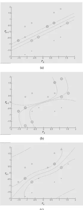
As shown in Fig. 4 and 5, SVM MUD with

Gaussian kernel functions show reasonably better

decision boundary than with other kernel

functions. In the simulation studies, SVM with

linear kernel functions didn't seem to be sensitive

with controlling parameter,



, while SVM with

both sigmoid and Gaussian did. It was found that

in the sigmoid case, the margin was getting

narrow with increase of



value. For Gausssian

kernel functons, the number of selected support

rk 1

rk₋

(a)

rk 1

rk₋

(b)

rk 1

rk₋

(c)

Fig. 5. Decision boundary with kernel functions Circled points: selected support vectors  , (a) Linear, (b) Sigmoid, (c) Gaussian

(a) 1+0.1z^-1

(b) 0.8+0.5z^-1+0.3z^-2 Fig. 3. Distribution of noise-free signals

(a)

(b)

(c)

Fig. 4. Decision boundary with kernel functions Circled points: selected support vectors ^{ }, (a) Linear, (b) Sigmoid, (c) Gaussian

vectors (SVs) was varying: 10 SVs with



 , 4

SVs with



   , while changing the shape

of decision boundary to the extent of selected

SVs. In Fig. 6, the error rate performance was

compared for two different channels. The bit error

rate (BER) performance was conducted with

100,000 inputs with Gaussian noise. The variance

(a) 1+0.1z^-1

(b) 0.8+0.5z^-1+0.3z^-2 Fig. 6. A comparison of error rate performance

parameter, 

^

used in Gaussian kernel functions is the same as noise variance estimated from



-means clustering techniques. As shown Fig. 6, the error rate performance of a SVM based MUD with Gaussian kernels outperforms with other kernels. This comes from the fact that the solution with Gaussian is approximately regarded as Bayesian optimal solution

^[7]

.

Ⅴ. Conclusion

The SVM based multiuser detector (MUD) described in this paper was investigated and analyzed with different kernel functions and SVM parameter. SVM MUD with linear kernels did not get influenced by controlling parameter,



_{. In} contrast, SVM MUD with both sigmoid and Gaussian kernel functions changed the number of SVs and the corresponding decision boundary

when the different



values were used. Also, It was found that SVM based MUD with the Gaussian Kernels performed better than the linear or sigmoid kernels.

Research has been continuing into more complex cases with higher channel order, many users, and long chip sequences. In addition, the another SVM training technique, the sequential mimimal optimization (SMO) will be investigated with different kernel functions, and its performance will be compared. Also, It is expected that the results of this study can be extended to various wireless cellular communication systems using multiple access schemes such as DS-CDMA, OFDM-CDMA, and multi-carrier CDMA.

References

[1] Madhow, U., Honig, M. L., “MMSE Interference Suppression for Direct Sequence Spread Spectrum CDMA,” IEEE Transactions on Communications, Vol.42., pp.3178-3188, 1994.

[2] Poor, H.V.,Verdu, S., “Probability of Errors in MMSE Multiuser Detection,” IEEE Transactions on Information Theory, Vol.43, pp.858-871, 1997.

[3] Aazhang, B., Paris, B.P., Orsak, G.C., “Neural Networks for Multiuser Detection in Code- Division Multiple-Access Channels,” IEEE Transactions on Communications, Vol.40, pp.1212-1222, 1992.

[4] Mitra, U., Poor, H.V., “Neural Network Techniques for Adaptive Multiuser Demodulation,” IEEE Journal on Selected Areas in Communications, Vol.12, pp.1460-1470, 1994.

[5] Cruickshank, D.G.M., “Radial Basis Function Receivers for DS-CDMA,” IEE Electronic Letters, Vol.32, pp.188-190, 1996.

[6] Matyjas, J.D., Psaromiligkos, I.N., Batalama, S.N., Medley, M.J., “Fast Converging Minimum Probability of Error Neural Network Receivers for DS-CDMA Communications,”

IEEE Transactions on Neural Networks, Vol.15,

pp.445-454, 2004.

[7] Chen, S., Mulgrew, B., Grant, P.M., “A Clustering Technique for Digital Communication Channel Equalization using Radial Basis Function Networks,” IEEE Transactions on Neural Networks, Vol.4, pp.570-579, 1993.

[8] Lee, J., Beach, C.D., Tepedelenlioglu, N., “A Practical Radial Basis Function Equalizer,”

IEEE Transactions on Neural Networks, Vol.10, pp. 450-455, 1999.

[9] Chen, S., Samingan, A. K., Hanzo, L., “Support Vector Machine Multiuser Receiver for DS-CDMA Signals in Multipath Channels”, IEEE Trans. on Neural Networks, Vol.12, pp.604-611, 2001.

[10] V. Vapnik, The Nature of Statistical Learning Theory. New York: Springer-Verlag, 1995.

[11] Burges, C. C. “A tutorial on support Vector Machine for Pattern Recognition,” Data Mining and Knowledge Discovery, Vol.2, pp.121-167, 1998.

이 정 식

(Jung-Sik Lee) 정회원

1983년 한양대학교 전자통신과 공학사

1990년 Florida Institute of Tech., Elec. Eng. M.S.

1996년 Florida Institute of Tech., Elec. Eng. Ph.D.

1997년～현재 군산대 전자정보 공학부 교수

2004년～2006년 미국 플로리다 주립대 (Univ. Of South Florida) 방문 교수

1986년～1988년 OPC 중앙연구소 연구원

<관심 분야> 적응신호처리,디지털 통신, 신경망응용

이 재 완

(Jae-Wan Lee) 정회원

1984년 중앙대학교 전자계산학 이학사

1987년 중앙대학교 전자계산학 이학석사

1987년 중앙대학교 컴퓨터공학 공학박사

1996년 3월～1998년 1월 한국 학술진흥재단 전문위원 1992년～현재 군산대학교 교수

<관심 분야>분산시스템, 운영체제.실시간, 컴퓨터 네트워크, 멀티미디어

황 재 정

(Jae-Jeong Hwang) 종신회원

한국통신학회 논문지 제 32권 8호 참조

정 경 택

(Kyung-Taek Chung) 종신회원

한국통신학회 논문지 제 24권 7호 참조