Comparison of linear and non-linear equation for the calibration of roxithromycin analysis using liquid chromatography/mass spectrometry

(1)

11

Comparison of linear and non-linear equation for the calibration of roxithromycin analysis using liquid chromatography/mass spectrometry

Jong-Hwan Lim

^1,2

, Hyo-In Yun

^1,

*

1

Research Institute of Veterinary Science, Chungnam National University, Daejeon 305-764

,

Korea

2

B&C Biopharm, Suwon 443-759, Korea

(Accepted: March 11, 2010)

Abstract : Linear and non-linear regressions were used to derive the calibration function for the measurement of roxithromycin plasma concentration. Their results were compared with weighted least squares regression by usual weight factors. In this paper the performance of a non-linear calibration equation with the capacity to account empirically for the curvature,

y

= a

x^b

+ c (b 1) is compared with the commonly used linear equation,

^y

= a

^x

+ b, as well as the quadratic equation,

^y

= a

^x²

+ b

^x

+ c. In the calibration curve (range of 0.01 to 10

µ

g/mL) of roxithromycin, both heteroscedasticity and non- linearity were present therefore linear least squares regression methods could result in large errors in the determination of roxithromycin concentration. By the non-linear and weighted least squares regression, the accuracy of the analytical method was improved at the lower end of the calibration curve. This study suggests that the non-linear calibration equation should be considered when a curve is required to be fitted to low dose calibration data which exhibit slight curvature.

Keywords : heteroscedastisity, LC/MS, non-linear calibration, roxithromycin

Introduction

A completely validated, accurate and reproducible bioanalytical method is an important requirement in pharmacokinetic and biopharmaceutical studies [2, 4, 6]. The quality of bioanalytical data is highly dependent on the quality of calibration model used to generate the standard curve; therefore, the choice of an appropriate calibration model is necessary for reliable quantification [4, 6]. However, unlike the pharmaceutical analysis, the concentration range in the bioanalysis test samples is dynamic, broad and normally of the order of three or more [4]. Although using two or more standard curves with different calibration ranges is common, a single standard curve that encompasses the entire dynamic concentration range in a pharmacokinetic study is of great use during routine analysis [4, 6].

Usually, linear models are preferable, but, if needed, the use of non-linear models should be considered [4, 18]. On the other hand, one of the basic assumptions

of the ordinary least squares regression method is constancy of variance or homoscedasticity for all response values [5, 6]. Many examples in analytical chemistry indicate that this assumption is not often fulfilled, i.e. the variability of the response often increases with the response level [6, 15]. In such a situation, some remedial actions like transformation or using weighted least regression must be done in order to stabilize the variance of the response and thus it can be accounted for heteroscedasticity [6, 15].

In such cases, an ordinary least square linear regression equation, by virtue of minimizing the residuals, gives less importance to the concentrations at or near the lowest limit of quantitation (LLOQ) and gives more importance in minimizing residuals at higher concen- trations [6]. This might result in incorrect measure- ments of unknown samples near the LLOQ and thus propose to question of the validity of the assay method.

Data transformations or the application of suitable weights are generally employed to overcome heterosce-

≠

*Corresponding author: Hyo-in Yun

Research institute of Veterinary Science, Chungnam National University, Daejeon 305-764, Korea

[Tel: +82-42-821-6759, Fax: +82-42-822-5780, E-mail: [email protected]]

(2)

dasticity [4, 6, 15].

Roxithromycin is an acid-stable oxime derivative of erytrhomycin which has similar

^{in vitro}

activity to erythromycin, but it is better absorbed after oral administration, and has a considerably longer half-life [3, 9, 13]. Various methods including high-performance liquid chromatography have been used to determine roxithromycin concentration in biological fluids for pharmacokinetic studies and therapeutic drug monitoring purposes [10, 11, 14, 17]. Most of the time, it is necessary to quantify roxithromycin over a wide concentration range in plasma or serum after adminis- tration of this drug. This fact can result in heteroscedasticity of response, so that the ordinary least squares regression methods cannot be used [10, 11, 14, 17]. The use of ordinary least squares regression in these situations could lead to the inaccurate estimation of roxithromycin concentration. In our previous studies, the calibration range of roxithromycin was divided into low and high concentration regions [10, 11].

The aim of the present study was to define a calibration function for determination of roxithromycin in dog plasma by a liquid chromatographic mass spectrometric (LC/MS) method over a 1,000-fold roxithromycin concentration range from 0.01 to 10

µ

g/mL. In this regard it was shown that the simple linear equation is not a suitable model. In addition, statistical methods such as linear and non-linear weighted least squares regression were evaluated to select the best model.

Materials and Methods

Chemicals

Roxithromycin as the standard was supplied by Shinil Biogen (Korea). HPLC grade methanol and acetonitrile were purchased from Mallinckrodt Baker (USA). Other analytical grade chemicals were purchased from Sigma (USA). Whole blood was obtained from healthy male beagle dogs.

Instruments and chromatographic conditions Samples were analyzed on a Hewlett-Packard 1100 series LC/MSD system. Separation was achieved on Watchers120 ODS-BP C

18

reverse phase column (5

µ

m, 4.6 mm × 150 mm; Daiso, Japan). Mobile phase composed of 20% of 10 mM ammonium acetate (pH 3.5) and 80% of acetonitrile. The column was held at ambient temperature and the flow rate was 0.8 mL/min.

The electrospray mass spectrometry (ES-MS) analysis was performed on a Hewlett-Packard 5989 electrospray mass spectrometer with a Hewlett-Packard atmospheric pressure ionization interface fitted with a hexapole ion guide. The instrument was tuned and optimized for the transmission of the nominal positive ion of roxithromycin (m/z 837.5). The optimal condition for the analysis of roxithromycin employed pneumatic nebulization with nitrogen (45 p.s.i.) and a counterflow of nitrogen (9 L/min) heated to 350

^o

C for the nebulization and desolvation of the introduced liquid.

Mass spectrometer was employed using the positive ion mode and the selected ion monitoring, detecting m/

z 837.5 with a dwell time of 300 ms.

Sample preparation and calibration standards A stock solution of 1,000

µ

g/mL roxithomycin was prepared in methanol and working calibration standards for five replicates at concentrations of 0.01, 0.1, 0.5, 1, 2.5, 5 and 10

µ

g/mL were prepared in blank plasma.

Plasma blank sample was analyzed in each run. Quality control (QC) samples were prepared at four different levels for three replicates, lower level (the LLOQ), low level (ten times LLOQ), middle level and high level (the upper limit of quantitation limit, ULOQ). QC samples were prepared daily by spiking different plasma samples to produce a final concentration equivalent to 0.01, 0.1, 5 and 10

^µ

g/mL of roxithromycin.

Sample preparation of roxithromycin was followed by the method of Lim

et al.

[10, 11] with some modifications. Briefly, to 200

^µ

L of spiked plasma, 10

µ

L of 2 N NaOH and 800

µ

L of ethyl acetate were added. To prevent the formation of an emulsion, extraction was performed gently for 10 min on a test- tube rotator. After centrifugation, the organic phase was transferred to tube and evaporated at 30

^o

C under a stream of nitrogen and then the residue dissolved in 200

^µ

L of 0.1% acetic acid in methanol. To the reconstituted sample, 800

µ

L of the

n

-hexane were added and vigorously shaken for 10 min. The lower layer was transferred to other tube and evaporated to dryness under a gentle stream of nitrogen at 37

^o

C. The dry extract was reconstituted in 40

^µ

L of the mobile phase, of which 10

µ

L was injected onto the chromato- graphic system.

Calibration models

Data analysis was conducted on the pooled data

(3)

using SPSS statistical packages. Variance test (

F

-test) was used in order to check for the presence of heteroscedasticity in the response data [6]. Because of the wide concentration range of roxithromycin, various types of models and weighting schemes were considered. The models were:

A:

y

= a

x

+ b B:

y

= a

x²

+ b

x

+ c C:

^y

= a

^x^b

+ c

where

y

is peak area of roxithromycin and

x

is roxithromycin concentration and a, b and c are parameters of the models. Weighting factors (w) were 1, 1/

x

, 1/

x²

, 1/

y

and 1/

y²

.

The best regression model and weighting factor was chosen according to the sum of absolute percentage relative error (%RE) values [1]. The %RE was compared with the regressed concentration (C

detected

) computed from the found regression equation obtained for each weighting factor, with the nominal standard concentration (C

nominal

):

The best model will be that which gives rise to a narrow horizontal band of randomly distributed %RE around the concentration axis and presents the least sum of the %RE across the whole concentration range.

Results

The homogenicity of response variance at different levels of roxithromycin was rejected through one-tailed

F

-test between highest and lowest concentrations of the calibration curve (

p

< 0.01). Also, examination of the studentized residual plots of various models without

%RE = C

^detected

C

nominal⁻

C

nominal

× 100

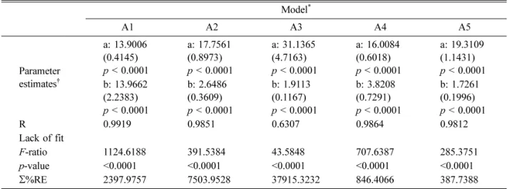
Table 1. Summary of the estimated parameters and results of lack-of-fit test for linear regression models (

^y

= a

^x

+b) fitted to data through weighted least squares regression using usual weight factors

Model

^*

A1 A2 A3 A4 A5

Parameter estimates

^†

a: 13.9006 (0.4145)

p

< 0.0001

a: 17.7561 (0.8973)

p

< 0.0001

a: 31.1365 (4.7163)

p

< 0.0001

a: 16.0084 (0.6018)

p

< 0.0001

a: 19.3109 (1.1431)

p

< 0.0001 b: 13.9662

(2.2383)

p

< 0.0001

b: 2.6486 (0.3609)

p

< 0.0001

b: 1.9113 (0.1167)

p

< 0.0001

b: 3.8208 (0.7291)

p

< 0.0001

b: 1.7261 (0.1996)

p

< 0.0001

R 0.9919 0.9851 0.6307 0.9864 0.9812

Lack of fit

F

-ratio 1124.6188 391.5384 43.5848 707.6387 285.3751

p

-value <0.0001 <0.0001 <0.0001 <0.0001 <0.0001

Σ

%RE 2397.9757 7503.9528 37915.3232 846.4066 387.7388

*

Linear regression models (

^y

= a

^x

+ b) fitted using weight factors 1 (A1), 1/

^x

(A2), 1/

^x²

(A3), 1/

^y

(A4) and 1/

^y²

(A5).

†

Standard error of parameter estimate is given in the first parenthesis below the parameter value.

Fig. 1. Studentized residual plots of the regression models fitted to data without weighting factor. (A)

^y

= a

^x

+ b; (B)

y

= a

x²

+ b

x

+ c; (C)

y

= a

x^b

+ c.

(4)

any weight factor confirmed the heterogeneity of variance (Fig. 1). Therefore, each model was fitted again to the pooled data using weighted least squares regression.

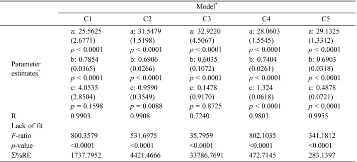
The estimated parameters and the result of lack of fit test for models fitted by weighted linear (or non-

linear) least squares regression method to data are shown in Table 1, Table 2 and Table 3. According to the results, models (A3, B3, C3) using weighting factor of 1/

^x²

should be discarded because of lower correlation coefficient,

R

, values (

R

< 0.8) or non-significance of parameters.

Table 2. Summary of the estimated parameters and results of lack-of-fit test for quadratic regression models (

y

= a

x²

+ b

^x

+ c) fitted to data through weighted least squares regression using usual weight factors

Model

^*

B1 B2 B3 B4 B5

Parameter estimates

^†

a: -0.2513 (0.0551)

p

< 0.0001

a: -0.546 (0.1079)

p

< 0.0001

a: -2.0892 (0.9541)

p

= 0.0325

a: -0.3982 (0.0685)

p

< 0.0001

a: -0.6955 (0.1608)

p

< 0.0001 b: 18.2044

(1.0119)

p

< 0.0001

b: 23.2533 (1.3294)

p

< 0.0001

b: 38.789 (5.7661)

p

< 0.0001

b: 20.6791 (0.942)

p

< 0.0001

b: 24.1742 (1.515)

p

< 0.0001 c: 8.6594

(2.2827)

p

= 0.0003

c: 2.434 (0.311)

p

< 0.0001

c: 1.8275 (0.1198)

p

< 0.0001

c: 3.0765 (0.6095)

p

< 0.0001

c: 1.6214 (0.1789)

p

< 0.0001

R 0.9888 0.9968 0.6626 0.9715 0.9942

Lack of fit

F

-ratio 741.1496 281.5199 25.4427 546.5847 190.3029

p

-value <0.0001 <0.0001 <0.0001 <0.0001 <0.0001

Σ

%RE 2081.6697 6339.7829 36167.9266 704.7675 352.7847

*

Quadratic regression models (

^y

= a

^x²

+ b

^x

+ c) fitted using weight factors 1 (B1), 1/

^x

(B2), 1/

^x²

(B3), 1/

^y

(B4) and 1/

^y²

(B5).

†

Standard error of parameter estimate is given in the first parenthesis below the parameter value.

Table 3. Summary of the estimated parameters and results of lack-of-fit test for power regression models (

^y

= a

^x^b

+ c) fitted to data through weighted least squares regression using usual weight factors

Model

^*

C1 C2 C3 C4 C5

Parameter estimates

^†

a: 25.5625 (2.6771)

p

< 0.0001

a: 31.5479 (1.5198)

p

< 0.0001

a: 32.9220 (4.5067)

p

< 0.0001

a: 28.0603 (1.5545)

p

< 0.0001

a: 29.1325 (1.3312)

p

< 0.0001 b: 0.7854

(0.0365)

p

< 0.0001

b: 0.6906 (0.0266)

p

< 0.0001

b: 0.6035 (0.1072)

p

< 0.0001

b: 0.7404 (0.0261)

p

< 0.0001

b: 0.6903 (0.0318)

p

< 0.0001 c: 4.0535

(2.8504)

p

= 0.1598

c: 0.9590 (0.3549)

p

= 0.0088

c: 0.1478 (0.9170)

p

= 0.8725

c: 1.324 (0.0618)

p

< 0.0001

c: 0.4878 (0.0721)

p

< 0.0001

R 0.9903 0.9908 0.7240 0.9803 0.9955

Lack of fit

F

-ratio 800.3579 531.6975 35.7959 802.1035 341.1812

p

-value <0.0001 <0.0001 <0.0001 <0.0001 <0.0001

Σ

%RE 1737.7952 4421.4666 33786.7691 472.7145 283.1397

*

Power regression models (

^y

= a

^x^b

+ c) fitted using weight factors 1 (C1), 1/

^x

(C2), 1/

^x²

(C3), 1/

^y

(C4) and 1/

^y²

(C5).

†

Standard error of parameter estimate is given in the first parenthesis below the parameter value.

(5)

The best fitting regression model and weighting factor was chosen taking in to account the sums of the

%RE calculated for the each regression model. The regression models with the 1/

y²

weighting factor produced relatively smaller %RE sum, and the most random distribution around the x-axis at the lower end of the calibration curve. Reconsideration of residual plots for all of the weighted regression models with weighting factor 1/

y²

showed that the use of these weight factors could lead to stabilization of variance (Fig. 2). The power regression equation with weighting factor 1/

y²

produced the least sum of %RE for roxithromycin calibration data set providing the most adequate approxi- mation of variance. Therefore, this model was used for determination of roxithromycin as calibration curve.

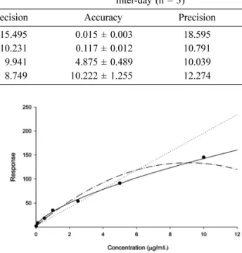
Seven concentrations of roxithromycin from 0.01 to 10

µ

g/mL in dog plasma were prepared to calibrate the instrument. Peak area of roxithromycin was used for regression and the standard curves were fitted to a 1/

y²

weighted power regression, where y represents the peak area of roxithromycin (Fig. 3). The accuracy and precision of the back-calculated concentrations were excellent. The limit of quantitation was defined as the lowest standard on the calibration curve as analyte peaks by which both compounds in blank plasma were identifiable, discrete and reproducible with a precision of 20% and accuracy of 80-120%. The validation data on the precision and accuracy for three replicates of QC samples are summarized in Table 4. These precision and accuracy values indicated reproducible LC/MS conditions and that the assay is consistent and reliable.

Discussion

Unlike pharmaceutical analysis, the concentration ranged in bioanalytical methods is usually dynamic and broad, presenting three or more orders of magnitude, Table 4. Inter- and intra-day accuracy and precision for the determination of roxithromycin in Beagle dog plasma

Nominal conc. (ìg/mL) Intra-day (n = 3) Inter-day (n = 3)

Accuracy Precision Accuracy Precision

0.01 0.011 ± 0.002 15.495 0.015 ± 0.003 18.595

0.1 0.124 ± 0.013 10.231 0.117 ± 0.012 10.791

5 5.445 ± 0.541 9.941 4.875 ± 0.489 10.039

10 10.130 ± 0.886 8.749 10.222 ± 1.255 12.274

Fig. 2. The residual plots for the weighted regression models with weighting factor 1/

^y²

. (A)

^y

= a

^x

+ b; (B)

^y

= a

^x²

+ b

^x

+ c; (C)

^y

= a

^x^b

+ c.

Fig 3. Comparison of the calibration curves using linear regression and non-linear regression model with weighting factor 1/

^y²

. (A) Dotted line,

^y

= a

^x

+ b; (B) Dash-dot line,

y

= a

^x²

+ b

^x

+ c; (C) Solid line,

^y

= a

^x^b

+ c.

(6)

in order to monitor concentrations effectively [2, 4, 7].

When the range in data values is large, it might be expected that variance of each data point might be quite different (heteroscedastic). Linear regression by the least square method assumes that each data point in the range has a constant absolute variation, however, many analytical methods produce data which are heteroscedastic in that the errors are a constant relative value [4, 7, 15]. The use of linear least squares regression in the construction of calibration curve with a very wide concentration ranges could lead to inaccurate estimation of concentration. In the present studies, both heteroscedasticity and non-linearity were observed in the calibration curve of roxithromycin ranging from 0.01 to 10

µ

g/mL. Least square linear regression without weight factors could result in large errors in the calculation of roxithromycin concentration.

Residual plots can be used to evaluated the need for weighting factor when unweight least square linear regression is applied [4, 6, 7]. If the data adequately fit the linear model, then the residuals should be randomly distributed in a horizontal band centered on the concentration axis [7]. In this study, the residual plots for unweighted regression clearly showed that the residuals were not randomly distributed around the concentration axis. Instead, an increase in variance as a function of concentration, heteroscedasticity, was observed. Usually, the use of weighted regression is recommended for heteroscedastic data, therefore weighted regressions for linear or non-linear regression models were performed in order to select a reasonable regression model for roxithromycin calibration data set.

Some curve-selection criteria involve evaluating the appropriateness of a given curve by comparing its goodness-of-fit relative to the rest of the models under consideration [8]. The simplest and most commonly used goodness-of-fit criterion is the multiple correlation coefficients, also called the correlation coefficient,

^R

. However, it is questionable whether

R

is the most appropriate criterion for model selection [8, 12]. Its blind use could lead to wrong deductions about the functional relationship between response and concentration [12]. In this study, some models clearly underestimated the concentrations in the lower range of the calibration curve, although they were shown high values of

R

. Therefore, the best weighting factor and fitted regression model were chosen according to the sum of the %RE calculated for each regression model. Among

of fitted regression models, the power regression equation (

y

= a

x^b

+ c) with weighting factor 1/

y²

produced the least value for sum of the %RE in roxithromycin calibration curve providing the most adequate approximation of variance. Using this calibration equation, the accuracy and precision of the back- calculated concentrations were excellent. For selected calibration equation in the present study, the correlation coefficient (

R

) of calibration fell in specified range (

R

> 0.955), and the y-intercepts were virtually zero, indicating the absence of endogenous interference.

Conclusion

In this work, the calibration model was chosen during validation. Although the choice of the calibration model is currently normally included in the pre- validation phase, it has been more recently recommended to include it during the validation procedure, by using all validation samples and individual calibration curves in several batches in order to simulate the real conditions of routine analysis [4, 7]. Szabo

et al

. [16]

also reported to a reduction of LOQ by using weighted linear analysis with improving precision and accuracy.

It is the utmost importance; the accurate quantitation of low plasma or serum concentrations versus time is particularly relevant in pharmacokinetic and pharma- codynamic studies. In addition, the present study for the selection of weighting and use of a complex regression equation may contribute to the justification required by the regulators, as it shows when, why and how to use weighting schemes for bioanalysts.

References

1. Almeida AM, Castel-Branco MM, Falcão AC.

Linear regression for calibration lines revisited:

weighting schemes for bioanalytical methods. J Chromatogr B Analyt Technol Biomed Life Sci 2002, 774 , 215-222.

2. Bressolle F, Bromet-Petit M, Audran M. Validation of liquid chromatographic and gas chromatographic methods. Applications to pharmacokinetics. J Chromatogr B Biomed Appl 1996, 686 , 3-10.

3. Bryskier AJ, Butzler JP, Neu HC, Tulkens PM.

Macrolides: Chemistry, Pharmacology and Clinical

Uses. pp. 167-182, Blackwell, Oxford, 1993.

(7)

4. Causon R. Validation of chromatographic methods in biomedical analysis. Viewpoint and discussion. J Chromatogr B Biomed Sci Appl 1997, 689 , 175-180.

5. Chow SC, Liu JP. Statistical Design and Analysis in Pharmaceutical Science. pp. 71-108, Marcel Dekker, New York, 1995.

6. Hartmann C, Smeyers-Verbeke J, Massart DL, McDowall RD. Validation of bioanalytical chromato- graphic methods. J Pharm Biomed Anal 1998, 17 , 193- 218.

7. Karnes HT, March C. Calibration and validation of linearity in chromatographic biopharmaceutical analysis.

J Pharm Biomed Anal 1991, 9 , 911-918.

8. Kimanani EK. Bioanalytical calibration curves:

Proposal for statistical criteria. J Pharm Biomed Anal 1998, 16 , 1117-1124.

9. Lassman HB, Puri SK, Ho I, Sabo R, Mezzino MJ.

Pharmacokinetics of roxithromycin (RU 965). J Clin Pharmacol 1988, 28 , 141-152.

10. Lim JH, Jang BS, Lee RK, Park SC, Yun HI.

Determination of roxithromycin residues in the flounder muscle with electrospray liquid chromatography-mass spectrometry. J Chromatogr B Biomed Sci Appl 2000, 746 , 219-225.

11. Lim JH, Park BK, Yun HI. Determination of roxithromycin by liquid chromatography/mass spectro- metry after multiple-dose oral administration in broilers.

J Vet Sci 2003, 4 , 35-39.

12. Montgomery DC, Peck EA. Introduction to Linear Regression Analysis. pp. 131-165, Wiley, New York, 1994.

13. Omura S. Macrolide Antibiotics: Chemistry, Biology,

and Practice. pp. 370-372, Academic Press, Amsterdam, 2002.

14. Qi M, Wang P, Cong R, Yang J. Simultaneous determination of roxithromycin and ambroxol hydro- chloride in a new tablet formulation by liquid chromatography. J Pharm Biomed Anal 2004, 35 , 1287-1291.

15. Sadray S, Rezaee S, Rezakhah S. Non-linear heteroscedastic regression model for determination of methotrexate in human plasma by high-performance liquid chromatography. J Chromatogr B Analyt Technol Biomed Life Sci 2003, 787 , 293-302.

16. Szabo GK, Browne HK, Ajami A, Josephs EG.

Alternatives to least squares linear regression analysis for computation of standard curves for quantitation by high performance liquid chromatography: applications to clinical pharmacology. J Clin Pharmacol 1994, 34 , 242-249.

17. Taninaka C, Ohtani H, Hanada E, Kotaki H, Sato H, Iga T. Determination of erythromycin, clarithromycin, roxithromycin, and azithromycin in plasma by high- performance liquid chromatography with amperometric detection. J Chromatogr B Biomed Sci Appl 2000, 738 , 405-411.