1. INTRODUCTION
Computing the nearest, farthest, or some inter- mediate neighbors is a fundamental problem in computational geometry and location-based serv- ices (LBS), and the results of these computations can be applied to many applications. Given a set of data points {⋯} in a spatial network, the farthest neighbor of a data pointp in P is de- fined as max{∈}, where is the length of the shortest path between two data points p and s. The problem of computing the farthest neighbor of each data point in P is referred to as the all-farthest-neighbors (AFN) search problem, which is the logical opposite of the all-nearest- neighbors (ANN) search problem [1, 2].
Nearest neighbor search has been studied ex- tensively, because of its importance and over- whelming impact in LBS [1-4]. However, little at- tention has been paid to farthest neighbor search,
even though it has real-life applications in a large number of fields, including marketing, facility loca- tion, clustering, and recommendation systems. Let us consider some real-life scenarios in which far- thest neighbor search is valuable. For example, if a user wants to purchase a facility that has a suffi- cient service range, such as a transceiver or tele- scope, the user can use the distance to the farthest neighbor to determine which facility to buy. In ad- dition, in contrast to the nearest neighbor, the far- thest neighbor can be of particular interest to a user just because of its remoteness. A farthest neighbor search can be used, for example, to de- termine the quiet places farthest from a noisy factory. Some tourists may be interested in the greatest distance between two cities in a country that can be traversed on land.
Fig. 1 shows an example of an AFN query in a spatial network, where data points p1 throughp5
denote places such as service stations. In this ex-
Efficient Processing of All-farthest-neighbors Queries in Spatial Network Databases
Hyung-Ju Cho†
ABSTRACT
This paper addresses the efficient processing of all-farthest-neighbors (AFN) queries in spatial network databases. Given a set of data points {⋯} in a spatial network, where the distance between two data points p and s, denoted by , is the length of the shortest path between them, an AFN query is defined as follows: find the farthest neighbor ∈ of each data point p such that
≥ for all ∈. In this paper, we propose a shared execution algorithm called FAST (for All-Farthest-neighbors Search in spatial neTworks). Extensive experiments on real-world roadmaps confirm the efficiency and scalability of the FAST algorithm, while demonstrating a speedup of up to two orders of magnitude over a conventional solution.
Key words: All-farthest-neighbors Query, Maximum Distance, Spatial Network Database
※ Corresponding Author : Hyung-Ju Cho, Address:
(37224) Gyeongsang-daero 2559, Sangju-si, Gyeongsang- buk-do, Republic of Korea, TEL : +82-54-530-1455, FAX : +82-54-530-1459, E-mail : [email protected] Receipt date : July 29, 2019, Revision date : Oct. 24, 2019
Approval date : Nov. 19, 2019
†Department of Software, Kyungpook National University
※ This work was supported by the National Research Foundation of Korea (NRF) grant funded by the Korean government (MSIP) (NRF-2019R1H1A2080073)
ample, the AFN query retrieves the farthest neigh- bor, denoted by, of each data pointp in P. We can compute the query result {〈〉∈}
{〈〉〈〉〈〉〈〉〈〉}. Unfortu- nately, few studies have been carried out on the AFN search problem [5, 6]. Baeet al. [6] proposed an efficient solution to AFN search in theL1plane with the Manhattan metric, in the presence of highways and obstacles. However, this approach cannot be extended to AFN search over spatial networks, because of inconsistencies in problem requirements between the L1 plane and a spatial network. Spatial queries based on farthest neigh- bor search have gained significant attention in re- cent years in the form of farthest neighbor queries [7], reverse farthest neighbor queries [8, 9], and aggregate farthest neighbor queries [10, 11]. How- ever, existing solutions cannot be readily applied to AFN queries in spatial networks because of dif- ferences in the problem specification and distance metrics.
The simplest search algorithm for AFN queries in spatial networks involves computing the network distance between every ordered pair〈〉∈ ×, which corresponds to the all-pairs-shortest-path problem [12], and then spending additional time to choose the farthest ordered pairs among all pairs in ×. This simple solution is too com- putationally expensive to be of any practical use, particularly for large datasets, because of the very large number of distance computations required between data points in spatial networks of even
moderate size. Therefore, we propose a new algo- rithm called FAST, for All-Farthest-neighbors Search in spatial neTworks. Our proposed solution is to cluster adjacent data points into a group and then optimize shared computation for the group, to rapidly filter candidates by computing the max- imum distance between two groups. Although the shared computation of spatial queries has received much attention [13-15], no shared computation strategy has been applied to AFN queries in spatial networks to date. In this study, we optimize the shared execution strategy to process AFN queries in spatial networks. The FAST algorithm is easy to implement, facilitating its integration with popu- lar network distance algorithms, such as transit node routing (TNR) [16] and G-tree [17], for spa- tial networks. We summarize the main contribu- tions of this study as follows.
∙ We propose an efficient algorithm, called FAST, that exploits the shared execution of groups to minimize the number of network distance computations.
∙ We present a mathematical formula to compute the maximum distance between two groups. We also present effective pruning techniques based on the maximum distance between the two groups.
∙ We conduct experiments under several different sets of conditions to demonstrate the efficiency and scalability of the FAST algorithm and dem- onstrate speedups of up to two orders of magni- tude over a conventional solution.
The remainder of this paper is organized as follows. In Section 2, we review related research.
In Section 3, we provide essential background knowledge. In Section 4, we present a method for converting adjacent data points into a group, and detail how to compute the maximum distance be- tween two groups. In Section 5, we present the FAST algorithm for performing AFN queries in Fig. 1. Example of an AFN query in a road network
where {}.
spatial networks using shared execution of the network distance computations. In Section 6, we report a comprehensive experimental study com- paring the FAST algorithm with a conventional solution under different circumstances. Finally, we discuss our conclusions in Section 7.
2. RELATED WORK
Many studies have been performed on the proc- essing of sophisticated spatial queries based on farthest neighbor search. Curtinet al. [7] presented an approximate farthest neighbor search algorithm that selects a set of candidate data points using data distributed in Euclidean space. They also de- veloped an information-theoretic entropy measure to investigate the difficulty of the farthest neighbor search problem. Luet al. [18] formulated the far- thest dominated location query, which retrieves a location such that the distance to its nearest domi- nating object is maximized, for spatial decision support applications. Gao et al. [10] and Wang et al. [11] studied aggregate k-farthest neighbor queries in Euclidean space and spatial networks, respectively. Given a set of data points P and a set of query data pointsQ, an aggregate k-farthest neighbor query returns thek data points in P that have the largest aggregate distances to all query data points inQ. Reverse farthest neighbors quer- ies have also been studied, both in Euclidean space [8, 9] and in spatial networks [19, 20]. Yaoet al.
[9] first studied reverse farthest neighbor query problem in Euclidean space. They proposed pro- gressive farthest cell and convex hull farthest cell algorithms to support reverse farthest neighbors queries using the R-tree [21]. Wanget al. [8] pre- sented a solution to support reverse k-farthest neighbors queries in Euclidean space for arbitrary values ofk. Tran et al. [19] studied reverse farthest neighbor queries in spatial networks using network Voronoi diagrams and precomputed network dis- tances. Xuet al. [20] presented efficient algorithms
based on landmarks and hierarchical partitioning to process monochromatic reverse farthest neigh- bors queries, as well as bichromatic reverse far- thest neighbors queries, in spatial networks. How- ever, existing solutions in Euclidean space cannot be readily applied to our situation because it is very difficult to exploit R-trees and convex hulls in spa- tial networks.
The AFN search problem has been recently ex- amined from a theoretical point of view [6, 22]. Bae et al. [6] proposed an efficient algorithm for AFN search in theL1plane in the presence of highways and obstacles. This approach cannot be extended to AFN search in spatial networks, because of in- consistent problem requirements. Daescu et al. [22]
presented solutions to farthest-point problems in the plane and showed how the solutions can be used to efficiently solve other complex problems, such as simplifying polygonal paths or determining the data point farthest from a query segment.
Katoh and Iwano [23] addressed the problems of enumerating the k closest or farthest bichromatic pairs of red and blue data points in the Euclidean space. However, large-scale spatial networks need practical and efficient algorithms for the evaluation of AFN queries, which limits the application of these theoretical approaches [6, 22] in our situation.
To process a large number of queries in a data- base system, the shared execution strategy has at- tracted considerable attention, because of its low processing cost [13-15]. The key idea of shared query execution is to cluster queries that share some common execution path into a group, and then execute the group as a single query in the system. These shared execution methods have been found to be effective in many applications in- volving high load conditions. In this study, we ex- ploit a shared execution strategy to increase the efficiency of AFN queries in spatial networks. Our proposed solution differs from existing studies in several ways. First, it represents the first attempt to evaluate AFN queries efficiently in spatial
networks. Second, it employs a shared execution strategy to rapidly filter candidates while process- ing AFN queries. Finally, it can be implemented easily using popular network distance algorithms [16, 17] in spatial networks, a highly desirable property in practice. A brief survey and empirical comparison of some of the most popular network distance algorithms are presented in [24]. The techniques presented in [1, 2, 17, 25] for nearest neighbor search cannot be directly applied to far- thest neighbor search, because the nearest neigh- bor search and farthest neighbor search have op- posite goals.
3. PRELIMINARIES
We first define the principal terms related to far- thest neighbor and AFN queries, and summarize the notation used in this paper.
Definition 1. (Farthest neighbor): The farthest neighbor of a data pointp from a set of data points P is defined as such that ∈ and
≥ for ∀∈. Ties are broken arbitrarily.
Definition 2. (AFN query): Given a set of data points P, an AFN query retrieves a set of ordered pairs, each consisting of a data point p in P and its farthest neighbor . The AFN query result
is formally defined as {〈〉∈}.
Definition 3. (Spatial network): We represent a spatial network as an undirected weighted graph
, where V is the set of vertices, E is the set of edges, and the weight → asso- ciates each edge with a positive real number repre- senting the network distance or travel time. Each data pointp is located on an edge in the spatial network.
Definition 4. (Classification of vertices): We di- vide vertices into three categories based on their degree. (1) If the degree of a vertex is greater than or equal to three, the vertex is referred to as an intersection vertex. (2) If the degree is two, the vertex is an intermediate vertex. (3) If the degree is one, the vertex is a terminal vertex.
Definition 5. (Vertex sequence and segment):
A vertex sequence ⋯ denotes a path be- tween two vertices vl and vm, such that each of vlandvmis either an intersection vertex or a termi- nal vertex, and the other vertices in the path,
⋯ , are intermediate vertices. The length of a vertex sequence is the total weight of the edges in the vertex sequence. A part of a vertex sequence is referred to as a segment. By definition, a vertex sequence is also a segment. Table 1 pres- ents the symbols and notation used throughout the
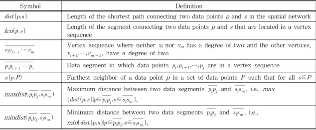
Table 1. Symbols and their meanings
Symbol Definition
Length of the shortest path connecting two data pointsp and s in the spatial network len Length of the segment connecting two data pointsp and s that are located in a vertex
sequence
⋯ Vertex sequence where neither vl nor vmhas a degree of two and the other vertices,
⋯ , have a degree of two
⋯ Data segment in which data points ⋯ are in a vertex sequence
Farthest neighbor of a data point p in a set of data points P such that for all ∈
maxdist( ) Maximum distance between two data segments and , i.e., max {∈∈},
mindist( ) Minimum distance between two data segments and , i.e., min{∈∈},
paper. To simplify the presentation, we use to denote ⋯ and use to denote
when P denotes the set of all data points.
4. PROCESSING AFN QUERIES IN SPATIAL NETWORK DATABASES
4.1 Grouping adjacent data points in a vertex sequence
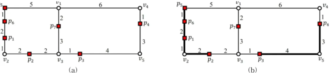
Fig. 2 presents an example of an AFN query in a spatial network, which will be used as the exam- ple throughout this section. As shown in Figure 2(a), given a set of data points {⋯}, an AFN query retrieves the farthest neighbor of each data point p in P . Fig. 2(b) shows the sample grouping of adjacent data points in a vertex sequence. As shown in Fig. 2(b), four data points p1, p2, p5, and p6 in a vertex sequence are grouped into a segment and two data pointsp3and p4in a vertex sequence are grouped into another segment . Naturally, the data pointp7in vertex sequence is not grouped because there is no other data point in the vertex sequence . Therefore, a set of data points {⋯} can be transformed into a set of seg- ments { }.
4.2 Computation of the distance between two segments
In this section, we describe the computation of the minimum and maximum distances between two data segments, and , which are de-
noted as mindist( ) and maxdist( ), respectively. Clearly,mindist( ) and maxd- ist( ) are formally defined as mindist ( )=min{∈∈} and maxd- i s t ( ) =m a x { ∈∈} , respectively.
Corollary 1. mindist( ) is a lower bound (maxdist( ) is an upper bound) on the dis- tance between two data points ∈ and ∈. Therefore, mindist( )≤ ≤maxdist ( ) for ∀∈ and ∀∈. ■
We describe how to compute mindist( ) and maxdist( ). If there exists an overlap between and (i.e.,∩≠ ∅), the min- imum distance between and is mindist ( )=0; otherwise, the minimum distance between and is mindist( )=min {}. Unlike the computation ofmindist( ), it is not intuitive to compute maxdist( ). We first describe how to compute the maximum distance between a segment and a data points in . For this, we investigate the distance between two data points p and s where ∈ and ∈.
In Fig. 3, let us assume that the data point pi
corresponds to the origin of the XY coordinate system. The X-axis and Y-axis then represent len
and , respectively, where ∈. For convenience, data pointp is represented by a rec- tangle, whereas data point s is represented by a
(a) (b)
Fig. 2. Grouping adjacent data points in a vertex sequence. (a) {⋯} (b) { }.
triangle. If there is a path from data pointp to data points via pi (i.e., →→), the distance between p and s is computed as len
, as shown in Fig. 3(a). Similarly, if there is a path fromp to s via pj(i.e., →→), then is computed as len
, as shown in Fig. 3(b). If the data points is located in , then is computed as len , as shown in Fig. 3(c).
Because is the length of the shortest path
among multiple paths between p and s, it is com- puted as follows:
Given a segment and a data point s, let
be the farthest data point ofs to a set of data points in , which means that there exists a data point s* in such that maxdist()
. We can then easily locates* in us-
(a) (b) (c)
Fig. 3. Determination of the distance from p to s where ∈. (a) len (b) len
(c) len.
(a)
(b) (c) (d)
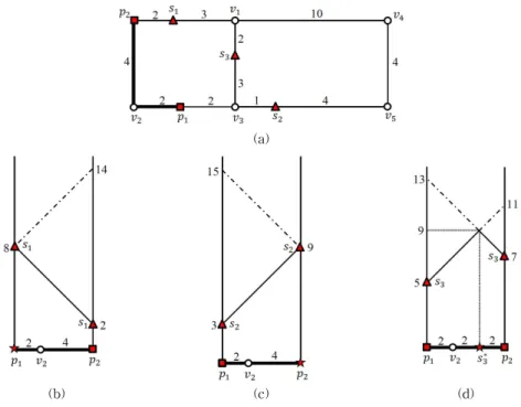
Fig. 4. Evaluation of maxdist(), maxdist(), and maxdist(). (a) Data segment and three data points s1, s2, and s3 (b) maxdist()=8 (c) maxdist()=9 (d) maxdist()=9.
ing the linear equation maxdist() . In Fig. 4, let us compute the farthest data point s* of each data point ∈{} such that
∈ and maxdist() . Because
, , len , and
len, we havemaxdist
and , as illustrated in Fig. 4 (b). Similarly, because , , len , and len, we havemaxdist and , as illustrated in Fig. 4(c). Finally, because
, , and len , the maximum distance between and is eval- uated asmaxdist and the farthest data point of is marked as in Fig. 4(d). The dash- ed/dotted lines in Fig. 4 indicate the lengths of re- dundant paths that are not the shortest.
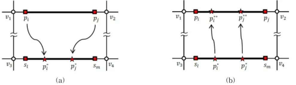
Fig. 5 illustrates the process of computingmaxd- ist( ). This process operates in two steps, which correspond to Fig. 5(a) and 5(b). In the first step, we find the farthest data point (respectively,
) of (respectively, ) such that (respectively, ), i.e.,maxdist
(respectively,maxdist ), as shown in Fig. 5(a). In the second step, we com- pute maxdist() and maxdist(), as shown in Fig. 5(b), where data point (respec- tively,
) indicates the farthest data point of
(respectively,
) such that
(respec-
tively, )-that is, maxdist
-as shown in Fig. 5(b). Returning to the example, let us compute the maximum distances of the three segments , , and in Fig.
2(b). Specifically, we evaluatemaxdist( ), maxdist(),maxdist(),maxdist(
), maxdist( ), and maxdist() in this order.
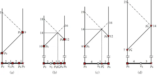
Fig. 6 illustrates how to compute maxdist ( ). As shown in Fig. 6(a), the maximum distance between and is evaluated as maxdist()=9 because we have
, , andlen . Therefore, the farthest data point of among is marked as
; that is, . As shown in Fig. 6(b), the maximum distance between and is evaluated asmaxdist()=14 be- cause we have , , and len . Therefore, the farthest data point of
among is marked as
; that is,
. As shown in Fig. 6(c), the max- imum distance between and is evaluated as maxdist()=14 because we have ,
, and len . Therefore, the farthest data point of among is marked as
; that is, . As shown in Fig. 6(d), the maximum distance between and
is eval- uated as maxdist()=14 because we have
(a) (b)
Fig. 5. Evaluation of maxdist( )=max{maxdist(), maxdist()}. (a) Finding and
(b) Evaluation of maxdist() and maxdist( ).
, , and len . Therefore, the farthest data point of among becomes ; that is,
. Consequently, the maximum distance between and is evaluated asmaxdist( )=max{
}=max{14,14}=14. Clearly, the minimum distance between and is evaluated as mindist( )=min
{}=
min{3,9,10,12}=3. Table 2 summarizes the mini- mum and maximum distances between the seg- ments in Fig. 2(b).
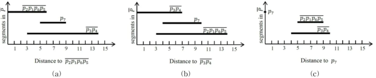
4.3 Sorting segments in decreasing order of their maximum distance
Fig. 7 illustrates sorting all segments in for each segment , for the example {
}. Specifically, the three segments in are sorted and plotted in decreasing order of the max- imum distance to each segment in . If segments with the same maximum distance are found, they are repeatedly sorted in decreasing order of their minimum distance. As shown in Fig. 7(a), , , and are sorted in this order for be- cause we have maxdist( )=14,maxdist ()=9, and maxdist( )=6.
(a) (b) (c) (d)
Fig. 6. maxdist( )=14. (a) maxdist()=9 and (b) maxdist()=14 and
(c) maxdist()=14 and (d) maxdist()=14 and .
Table 2. Minimum and maximum distances between pairs of segments in
maxdist( ) mindist( )
maxdist( )=6 maxdist( )=14 maxdist()=9
mindist( )=0 mindist( )=3 mindist()=5
maxdist( )=14 maxdist( )=7 maxdist()=10
mindist( )=3 mindist( )=0 mindist()=4
maxdist( )=9 maxdist( )=10 maxdist()=0
mindist( )=5 mindist( )=4 mindist()=0
As shown in Fig. 7(b), , , and are sorted in this order for because we have maxdist( )=14, maxdist()=10, and maxdist( )=7. Finally, as shown in Fig.
7(c), , , and are sorted in this order for because we have maxdist( )=10, maxdist( )=9, and maxdist()=0.
5. ALL-FARTHEST-NEIGHBORS SEARCH ALGORITHM OVER SPATIAL NETWORKS
Algorithm 1 describes the FAST algorithm for AFN search over spatial networks. The result set
is initialized to the empty set (line 1). In the first step, adjacent data points ⋯ in a vertex sequence are grouped into a data segment
and a set P of data points is converted to a set of segments, which is explained in Section 4.1 (lines 2-3). The AFN search is performed for each segment in to find the farthest neighbor
of each data point in the segment (line 6). The result of the AFN search for is added to the query result, where {〈〉∈} (line 7). Finally, the query result
is reported after the AFN search for all segments in is performed (line 8).
Algorithm 2 describes the AFN search algorithm for finding the farthest neighbor of each data point in . This algorithm sequentially traverses each of the sorted segments in . Note that all segments in are sorted in decreasing order of their max- imum distance to . First, the result set is initialized to the empty set (line 1). The pruning distance of each data point in is initialized to (line 2), where in- dicates the distance from to its most probable farthest neighbor. Similarly, the pruning distance of is the minimum pruning distance of all data points in ; that is, min {∈}. Based on Corollary 1, we pres-
Algorithm 1. FAST (P) Input: P: set of data points
Output: : set of ordered pairs of each data point ∈ and its farthest neighbor, i.e., {〈〉∈}.
1 ←∅ // the result set is initialized to the empty set.
2 // adjacent data points in each vertex sequence are grouped into a segment, as explained in Section 4.1.
3 ←group_points (P) // data points ⋯ in a vertex sequence are grouped into a data segment . 4 // for each data segment, it retrieves the FN of each data point in the segment, which is detailed in Algorithm 2.
5 for each segment ∈ do
6 ←AFN_search // {〈〉∈}.
7 ←∪ // the AFN search result for is added to .
8 return // is returned after the AFN search for each data segment ∈ is executed.
(a) (b) (c)
Fig. 7. Sorting all segments in decreasing order of their maximum distance to ∈{ }. (a) Sorting all segments for (b) Sorting all segments for (c) Sorting all segments for .
ent the following two corollaries to filter the re- maining unexplored segments, because these seg- ments can be safely neglected in the AFN search.
Corollary 2. Ifmaxdist( ) , the remaining unexplored segments can be safely ignored for the AFN search of the segment , because all segments in are sorted in decreasing order of their maximum distance to . ■
Corollary 3. Ifmaxdist() , the distance computation between data point and each data point in can be safely ignored for the AFN search of, because no data point in can be the farthest neighbor of . ■
All segments are explored sequentially to find the farthest neighbor of each data point in . Whenever a data segment is investigated, the pruning distance of is updated to the minimum
pruning distance of all data points in (line 9).
According to Corollary 2, if maxdist( )
, the AFN search algorithm termi- nates by returning the result set ; otherwise,
is explored to find the farthest neighbor of each data point in . According to Corollary 3, ifmaxdist() , no data point in can be the farthest neighbor of , and so the dis- tance computation between and all data points in can be safely ignored for ; otherwise, for each data point s in , we compute . If
, the farthest neighbor of and its pruning distance are updated to s and , respectively (lines 17-18). Accordingly, the prun- ing distance of is also updated to
. Finally, the result set is returned if maxdist( ) (lines 10-11) or Algorithm 2. AFN_search
Input: : data segment, : set of data segments
Output: : set of ordered pairs of each data point in and its farthest neighbor 1 ←∅ // the result set is initialized to the empty set.
2 ← for ∀∈ // the pruning distance of each data point p in is initialized to 0.
3 // the maximum and minimum distances from to each segment in are computed as explained in Section 4.2.
4 for each data segment ∈ do
5 compute maxdist( ) and maxdist( )
6 // all the segments in are sorted in decreasing order of their maximum distance to as explained in Section 4.3.
7 ←sort_by_dec_order ( ) // contains the sorted segments for the data segment . 8 for each data segment ∈ do
9 ←min{∈} // the pruning distance of is updated.
10 if maxdist( ) then // note that all the segments are sorted in decreasing order.
11 return // is returned if maxdist( ) .
12 else // it means that maxdist( )≥ .
13 for each data point ∈ do
14 if maxdist( )≥ then // is updated to .
15 for each data point ∈ do 16 if then
17 ← // the pruning distance of p is updated to .
18 ←∪{ 〈〉} −
{〈〉} // an updated ordered pair 〈〉 is added to 19 return // is returned if all segments in have been explored
if all segments in have been explored (line 19).
6. PERFORMANCE STUDY
In this section, we report the results of an em- pirical analysis of our proposed solution. We pres- ent our experimental settings in Section 6.1, fol- lowed by our experimental results in Section 6.2.
6.1 Experimental settings
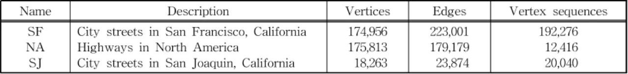
In the experiments, we use three real-world roadmaps [26], which are described in Table 3.
These real-world roadmaps have different sizes and each is a part of the US road network. Specifi- cally, the first roadmap includes major roads (such as city streets) in San Francisco (SF), California and corresponds to a data universe of approx- imately × km2. The second roadmap includes major roads (such as highways) in North America (NA) and corresponds to a data universe of ap- proximately × km2. The third roadmap in- cludes major roads (e.g., city streets) in San Joaquin (SJ), California and corresponds to a data universe of approximately × km2.
The experimental parameter settings are given in Table 4. For convenience, each dimension of the data universe is normalized independently to unit length . The data points have either centroid or uniform distributions. The centroid-based data- set is generated to resemble the real-world data.
First, five centroids are selected randomly. The da-
ta points around each centroid follow a normal dis- tribution, where the mean is set to the centroid and the standard deviation is set to 1% of the side length of the data universe.
In the performance study, we evaluated the per- formance of FAST using the query processing time. To the best of our knowledge, there is no competitive solution to efficiently evaluate AFN queries in spatial network databases, so we con- sidered a baseline method as a benchmark to verify the performance of the FAST method. The baseline method finds the farthest neighbor of each data point in P by computing the network distance be- tween every ordered pair 〈〉∈ × and then spending additional time to identify the farthest ordered pairs among all pairs in × . Both methods were implemented in C++ (Microsoft Visual Studio 2017), using common subroutines for similar tasks. We conducted experiments on a desktop computer running Windows 10 with a 4.2 GHz processor and 32 GB of memory. We believe that indexing structures of all techniques should be resident in memory to ensure responsive query processing; this is assumed in many recent studies [3, 24] and is crucial to commercial LBS as well as online map services. We determined the average values for each method based on repetitions of the experiments. Finally, we employed the TNR meth- od [16] to rapidly compute the network distance between two data points. According to the per- formance comparison in [24], the TNR method
Table 3. Real-world roadmaps
Name Description Vertices Edges Vertex sequences
SF NA SJ
City streets in San Francisco, California Highways in North America
City streets in San Joaquin, California
174,956 175,813 18,263
223,001 179,179 23,874
192,276 12,416 20,040
Table 4. Experimental parameter settings
Parameter Range
Number of data points () Distribution of data points Roadmap
500, 1000, 2000, 3000, 5000 (C)entroid, (U)niform SF, NA, SJ
achieves competitive performance regardless of the benchmark where it is tested.
6.2 Experimental results
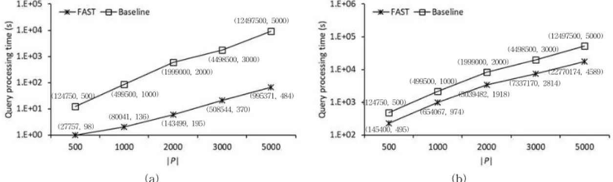
Fig. 8 shows a comparison of the query process- ing times of the FAST and baseline methods for the evaluation of AFN queries in the SF roadmap.
To evaluate the performance of the FAST method, we examined the number of network distance computations and data segments generated from adjacent data points for each experimental setup.
The two values in parentheses in Fig. 8, 9, and 10 indicate the number of network distance computa- tions performed by the FAST method and the number of data segments generated from adjacent data points. Similarly, we have also represented the number of network distance computations for the baseline method and the number of data points to Fig. 8, 9, and 10 for comparison. As shown in Fig.
8(a), the query processing time of the FAST meth- od for a centroid distribution of data points is less than that of the baseline algorithm by up to 22.8 times for . The difference in performance between the FAST and baseline algorithms tends to increase with because the FAST method ex- ploits the shared execution of AFN searches during the query evaluation. The shared execution of the FAST method aims to minimize the number of network distance computations. To do this, the FAST method groups the adjacent data points into a joint data segment and exploits shared computa- tion for this data segment to rapidly filter candi- dates by computing the maximum distance be- tween two data segments. Therefore, as the num- ber of data segments generated from the adjacent data points decreases, the difference between the FAST and baseline methods in terms of perform- ance increases. The query processing time of the
(28653, 94)
(169970, 264)
(407826, 412) (1396043, 456) (3383403, 1181) (124750, 500)
(499500, 1000) (1999000, 2000) (4498500, 3000)
(12497500, 5000)
(124750, 500) (499500, 1000)
(1999000, 2000)
(4498500, 3000) (12497500, 5000)
(130695, 499)
(519343, 999)
(2152608, 1997) (5075493, 2988)
(14940474, 4975)
(a) (b)
Fig. 8. Comparison of query processing time for SF roadmap. (a) Centroid distribution (b) Uniform distribution.
(58679, 142) (104434, 163)(555531, 152) (926651, 154)(729348, 277) (124750, 500)
(499500, 1000)
(1999000, 2000)(4498500, 3000) (12497500, 5000)
(174375, 467)
(721432, 863)
(3039834, 1616)(6422407, 2203)(15701885, 3261) (499500, 1000)
(1999000, 2000)
(12497500, 5000)
(124750, 500)
(4498500, 3000)
(a) (b)
Fig. 9. Comparison of query processing time for NA roadmap. (a) Centroid distribution (b) Uniform distribution.