TEXTURE ANALYSIS, IMAGE FUSION AND KOMPSAT-1
F.P. KRESSLER
1, Y.S. KIM
2, K.T. STEINNOCHER
11
ARC Seibersdorf research, Department for Environmental Planning, 2444-Seibersdorf, Austria [email protected]
2
Korea Aerospace Research Institute (KARI), Satellite Operation & Application Center, Yusung, Taejon, Korea
ABSTRACT
In the following paper two algorithms, suitable for the analysis of panchromatic data as provided by KOMPSAT-1 will be presented. One is a texture analysis which will be used to create a settlement mask based on the variations of gray values. The other is a fusion algorithm which allows the combination of high resolution panchromatic data with medium resolution multispectral data. The procedure developed for this purpose uses the spatial information present in the high resolution image to spatially enhance the low resolution image, while keeping the distortion of the multispectral information to a minimum. This makes it possible to use the fusion results for standard multispectral classification routines. The procedures presented here can be automated to large extent, making them suitable for a standard processing routine of satellite data.
Key words: texture analysis, image fusion, panchromatic, multispectral, KOMPSAT-1
1. INTRODUCTION
With the launch of KOMPSAT-1 and its EOC (Electo-Optical Camera) in 1999 a valuable data source became available. Two applications, which are ideally suited for panchromatic data will, be presented in this paper. One is a texture analysis, which allows the discrimination of image features on the basis of local variations of gray values. The other is an image fusion technique. This process allows the spatial enhancement of medium resolution multispectral data from sensors
such as Landsat TM and IRS-1C. This is done by combining the spatial information of the high resolution panchromatic data with the multispectral information of the medium resolution data. In this context care must be taken to keep the distortion of the multispectral information to a minimum. This is essential when classification procedures are to be applied to the fusion results.
In the next section the study area and the image data will be discussed. This is followed by a presentation of the texture analysis and results obtained from the analysis of KOMPSAT-1 data with special emphasis on the detection of urban areas. The next section examines image fusion and the results obtained for the same study area, as was examined with the texture analysis.
2. DATA AND STUDY AREA
For this study two data sets were available. One recorded by KOMPSAT-1 on 1
st, March 2001 the other by Landsat-7 ETM (Enhanced Thematic Mapper) on 10
th, September 2000. KOMPSAT-1 EOC records in one panchromatic band with a spectral resolution of 6.6 x 6.6 m, a radiometric resolution of 8-bit and a swath width of approximately 17 km per scene. The spatial resolution of the available scene was resampled to 6 m.
Landsat-7 ETM (Enhanced Thematic Mapper)
records reflected light in seven spectral bands, of which
six lie in the visible and infrared part of the spectrum and
one in the thermal part. The latter will not be used for the
analysis. The spatial resolution of the bands is
28.5 x 28.5 m, which was resampled to 30 x 30 m.
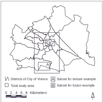
The study area lies in the capital of Austria, the City of Vienna (see Figure 1). Both texture analysis and fusion were carried out for the whole study area covering approximately 8.5 x 14 km.
0 2 4 6 8 Kilometers
N
Districts of City of Vi enna A Total study area
Subset for texture example Subset for fusion example B
A B
Figure 1: City of Vienna with Study Area
In order to visualize the results of the analysis two subsets were chosen, A (4.0 x 2.7 km) for the texture analysis and B (3.2 x 2.4 km) for the image fusion.
3. TEXTURE ANALYSIS 3.1. METHODOLGY
The high spatial resolution of satellite images acquired by sensors such KOMPSAT-1 EOC and IRS-1C/D panchromatic contain a large number of objects. For their recognition the human visual system does not only rely on the intensity of individual pixels but mainly on the spatial variations of these intensities, in general called texture. The method used here to derive textural features uses gray-level co-occurrence (GLC) matrices (Haralick et al., 1973). The GLC matrix contains estimates for the transition probabilities of the gray-level of two neighboring pixels. In order to obtain a texture feature image, the texture is calculated in a moving window for each pixel. The result is a digital image where single pixel values represent the degree of
texture in the local neighborhood. Considering the different texture features available, directions and distances that may be used and the variability of the size of the moving window, a great number of texture feature images can be derived from a single image. However, for most applications this can be reduced to a reasonable number of images. In terms of directions a minimum number of four is recommended, as they cover all distances that occur in a 3 x 3 neighborhood (horizontal, vertical and the two diagonals). In addition an appropriate window size has to be chosen. The minimum size of 3 x 3 has a similar effect as a edge detection filter.
As with all neighborhood algorithms the results will become smoother as the window size increases. At the same time the computational effort will increase exponentially.
Each texture image is calculated for a specific direction. In order to create a rotation invariant texture image which differentiates between homogenous and heterogeneous objects, the maximum difference of the different orthogonal texture features is first calculated. If this is subtracted from the average texture image calculated from all texture images, rotation invariant objects are preserved, while edges are removed. A detailed description and discussion of this method is given in Steinnocher (1997).
The creation of the settlement mask is carried out by
creating a binary image from the texture image by
introducing a threshold As this result will normally
contain some artifacts in the form of empty areas within
urban fabric as well as an overestimation of urban fabric
in rural areas an additional processing step can be
applied to smooth the result. This is first done by
shrinking areas identified as urban fabric, thus
eliminating very small areas, which are not part of
continuous urban fabric. Next a growing algorithm
allows the remaining areas to return to their original
form and also to fill smaller holes within the settlement
mask.
3.2. RESULTS TEXTURE ANALYSIS
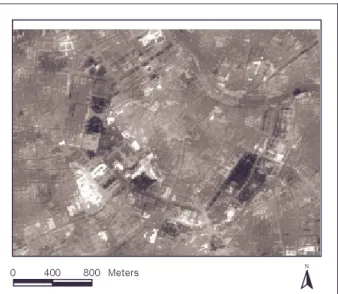
The algorithm described above was applied to the total study area. Subset A will be used to illustrate the results. Figure 2 shows the KOMPSAT-1 EOC image of this subset. It contains different cover types, ranging from agricultural and industrial/commercial areas to various types of residential areas.
͡ ͦ͡͡ ͢͡͡͡ ;ΖΥΖΣΤ N
Figure 2: KOMPSAT-1 Image of Subset A
In a first step the texture analysis was applied to the satellite image with a window size of 9 x 9. This process involves first the calculation of all 4 directions (horizontal, vertical and the two diagonals). The final rotation invariant texture image (see Figure 3) was obtained by calculating the maximum difference of the different orthogonal texture images and subtracting the result from the average texture window.
͡ ͦ͡͡ ͢͡͡͡ ;ΖΥΖΣΤ N High texture
Low texture
Figure 3: Result of Texture Analysis for Subset A
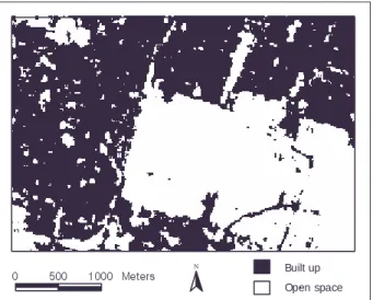
Rotation invariant objects (shown in dark tones) remain and are an indication of the presence of settlements. In order to o create a mask the texture image was converted into a binary image by applying a threshold (see Figure 4). It can be seen that some artifacts such as holes in urban areas still remain.
͡ ͦ͡͡ ͢͡͡͡ ;ΖΥΖΣΤ N Built up
Open space
Figure 4: Binary Image created from Texture Image by applying a Threshold
Different ways exist to smooth the result. Here a morphological filter (Haralick, et al., 1987) with a window size of 5 x 5 was applied. The final result (see Figure 5), when compared with the original image, shows the settlement areas that have been identified, with some artifacts along a road network in the agricultural areas still remaining.
͡ ͦ͡͡ ͢͡͡͡ ;ΖΥΖΣΤ N Built up
Open space
Figure 5: Settlement mask after filtering Binary Image
4. ADAPTIVE IMAGE FUSION 4.1. METHODOLOGY
Fusion of multiresolution optical image data aims at the derivation of multispectral images providing the high spatial resolution of the panchromatic image. The perfect result of such a process would be an image, that is identical to the image the multispectral sensor would have observed if it had the high resolution of the panchromatic sensor (Wald et al., 1997).
In order to separate image objects, i.e. to assign each pixel to one of these objects, adaptive filter techniques can be uses. They allow the separation along the object edges based on the distribution of each object.
The sigma filter averages only those pixels in a local window, which lie in a two-sigma range of the central pixel value (Lee, 1983). All other pixels are assumed to belong to another distribution, i.e. they represent a neighboring object. As this filter is based on the assumption that the central pixel is in fact the mean of its Gaussian distribution, it might not include all relevant pixels in the averaging process. Therefore a more general approach, namely the modified sigma filter, was presented by Smith (1996). It averages all pixels, which could belong to the same distribution as the central pixel without knowing the actual mean of its distribution.
Application of the modified sigma filter requires the estimation of the normalized standard deviation which can be based on empirical analysis of the panchromatic image (Smith, 1996). First, a local average and a local standard deviation image are computed from the original image, using the window size chosen for the filter process. Next, the standard deviation image is divided by the average image on a pixel basis resulting in a normalized standard deviation image. When applying the modified sigma filter, areas with a low standard deviation, i.e. areas containing one object, will be smoothed. Within areas of high standard deviation, i.e.
areas containing object edges, only those pixels will be
averaged that belong to the same distribution as the central pixel.
The AIF algorithm starts by applying a modified sigma filter to the panchromatic image. At each position of the moving window the two sigma range related to the central pixel is calculated and all pixels within the window which fall into that range are selected. The position of the selected pixels is then transferred to the multispectral band, where the averaging of the respective sub-pixels is performed. Thus the filter behavior is controlled by the panchromatic band. No spectral information is transferred from the panchromatic image to the multispectral band during the whole procedure.
Thus the multispectral information is not significantly changed.
Although AIF sharpens the multispectral image according to object edges found in the panchromatic image, this effect is limited to object edges that occur both in the panchromatic as well as in the multispectral image. Edges appearing only in the panchromatic image will cause no significant effect in the multispectral band, while edges in the multispectral band that do not show up in the panchromatic image will be slightly blurred.
Objects that are smaller than the original multispectral pixel size will only be sharpened if their spectral reflectance is significantly different from their local environment. At the same time as object edges are sharpened, the area within an object will be smoothed.
4.2. RESULTS AIF
As an example the KOMPSAT-1 EOC scene was
fused with Landsat-7 ETM scene. A window size of 21
was considered to be suitable. It was found that by
applying the AIF iteratively better results could be
obtained. In our case three iterations were performed,
with the smoothed panchromatic and fusion results of
one run being the input of the next iteration. At each step
the fusion was further improved. Although the fusion
was applied to all 6 bands, only band three will be shown as an example.
Figure 6 shows the KOMPSAT-1 EOC image of the city center of Vienna. It is a densely built-up area with the Danube Canal in the Northeast and the Ringstrasse, a broad boulevard with a large number of parks, museums and theaters encircling the center.
͡ ͥ͡͡ ͩ͡͡ ;ΖΥΖΣΤ N
Figure 6: KOMPSAT-1 Image of Subset B
Band three of the Landsat-7 ETM-scene with a spatial resolution 30 x 30 m is shown in Figure 7. Although basic structures such as parks (shown very dark) and the shape of the Ringstrasse can be identified, interpretation is very limited.
͡ ͥ͡͡ ͩ͡͡ ;ΖΥΖΣΤ N
Figure 7: Subset of Band 3 Landsat-7 ETM
Figure 8 shows the result of the AIF after three iterations with a window size of 21 x 21. When compared with the original KOMPSAT scene it can be seen that most streets and even most courtyards can be identified. At the same time the multispectral information of the lower-resolution image is present as well.
͡ ͥ͡͡ ͩ͡͡ ;ΖΥΖΣΤ N