Semisupervised support vector quantile regression

Semisupervised support vector quantile regression ^†

Kyungha Seok ¹

1 Department of Statistics, Inje University

Received 11 February 2015, revised 11 March 2015, accepted 16 March 2015

Abstract

Unlabeled examples are easier and less expensive to be obtained than labeled exam- ples. In this paper semisupervised approach is used to utilize such examples in an effort to enhance the predictive performance of nonlinear quantile regression problems. We propose a semisupervised quantile regression method named semisupervised support vector quantile regression, which is based on support vector machine. A generalized ap- proximate cross validation method is used to choose the hyper-parameters that affect the performance of estimator. The experimental results confirm the successful perfor- mance of the proposed S2SVQR.

Keywords: Generalized approximate cross validation function, kernel trick, quantile regression, semisupervised learning, support vector machine.

1. Introduction

Quantile regression has been a popular method for estimating the quantiles of a conditional distribution of response variable given the values of input variables since Koenker and Bassett (1978) introduced the linear quantile regression. Just as classical linear regression methods based on minimizing sum of squared residuals enable us to estimate a wide variety of models for conditional mean functions, quantile regression methods offer a mechanism for estimating models for the full range of conditional quantile functions including the conditional median function. By supplementing the estimation of conditional mean functions with techniques for estimating an entire family of conditional quantile functions, quantile regression is capable of providing a better statistical analysis of the stochastic relationships among random variables.

The introductions and current research areas of the quantile regression can be found in Koenker (2005), Yu et al. (2003) and Shim and Hwang (2009).

Support vector machine (SVM) is being used as a new technique for regression and classi- fication problems. SVM is based on the structural risk minimization (SRM) principle, which has been shown to be superior to traditional empirical risk minimization (ERM) principle.

SRM minimizes an upper bound on the expected risk unlike ERM minimizing the error on the training data. By minimizing this bound, high generalization performance can be

† This research was supported by Basic Science Research Program through the National Research Foun- dation of Korea (NRF) funded by the Ministry of Education, Science and Technology with grant no.

(2011-0009705).

1

Professor, Institute of Statistical Information, Department of Statistics, Inje University, Kimhae 621-

749, Korea. E-mail: [email protected]

achieved. In particular, for the SVM regression case SRM results in the regularized ERM with the e-insensitive loss function. The introductions and overviews of recent developments of SVM can be found in Vapnik (1995, 1998), Smola and Sch¨ olkopf (1998), Wang (2005) and Hwang (2010).

In regression problem the labeled data implies real valued response variables and their corresponding input variables, and for classification problem the label indicates the class to which the corresponding data belongs. Most regression methods rely on the availability of large labeled data, since the larger the number of training data, the better the performance of the resulting regression methods. However, in practice, obtaining labeled data sometimes cost much. To overcome this problem, Blum and Mitchell (1988) proposed a co-training algorithm. Since then, researchers have studied the semisupervised learning principle - Chen et al. (2002), Wang et al. (2007) and Chapelle et al. (2008) proposed semisupervised learning methods using SVM, Zhang et al. (2009), Seok (2010) and Xu et al. (2011) proposed semisu- pervised learning methods using the least-squares SVM (Suykens and Vanderwalle, 1999).

Semi-supervised regression based local polynomial model, kernel ridge, and SVM were de- veloped (Seok, 2012, 2013, 2014). Those methods use large amounts of unlabeled data with small amounts of labeled data, and the empirical results confirm that unlabeled data can be used to significantly improve the predictive performance.

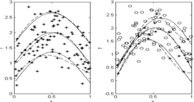
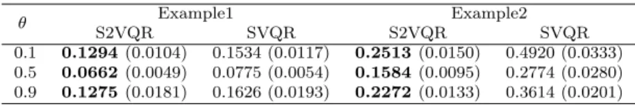
In this paper we derive a noble algorithm of semisupervised learning for support vector quantile regression (S2SVQR) based on support vector machine formulation. In Section 2 we review SVQR using check function. In Section 3 we propose S2SVQR using SVQR. In Section 4 we perform the numerical studies through examples. In Section 5 we give the conclusions.

2. Support vector quantile regression

Let the training data set denoted by {(x i, y i )} ⁿ _i=1 , with each input x i ∈ R ^d and the response y i ∈ R, where the output variable y i is linearly or nonlinerly related to the input vector x i . Here the feature mapping function φ(·) : R ^d → R ^d

maps the input space to the higher dimensional feature space where the dimension d f is defined in an implicit way.

An inner product in feature space has an equivalent kernel in input space, φ(x i ) ⁰ φ(x j ) = K(x i , x j ) (Mercer, 1909). Several choices of the kernel K(·, ·) are possible. We consider the nonlinear regression case, in which the quantile regression function q(x) of the response given x can be regarded as a nonlinear function of input vector x.

With a check function ρ _θ (·), the estimator of the θth quantile regression function can be defined as any solution to the optimization problem,

min 1

2 w ⁰ w + C

n

X

i=1

ρ _θ (y _i − q(x _i ))

where ρ θ (r) = θrI _(r>=0) + (1 − θ)rI _(r<0) . We can express the quantile regression problem by formulation of SVM as follows:

min 1

2 w ⁰ w + C

n

X

i=1

(θξ i + (1 − θ)ξ _i ^∗ )

subject to

y i − w ⁰ φ(x i ) − b ≤ ξ i , w ⁰ φ(x i ) + b − y i ≤ ξ _i ^∗ , ξ i , ξ _i ^∗ ≥ 0, where C > 0 is a penalty parameter penalizing the training errors.

We construct a Lagrange function as follows:

L = 1

2 w ⁰ w + C

n

X

i=1

(θξ i + (1 − θ)ξ ^∗ _i ) −

n

X

i=1

α i (ξ i − y i + w ⁰ φ(x i ) + b) (2.1)

−

n

X

i=1

α ^∗ _i (ξ _i ^∗ + y i − w ⁰ φ(x i ) − b) −

n

X

i=1

(η i ξ i + η ^∗ _i ξ _i ^∗ ).

We notice that the positivity constraints α i , α ^∗ _i , η i , η ^∗ _i ≥ 0 should be satisfied. After taking partial derivatives of equation (2.1) with regard to the primal variables (w, b, ξ i , ξ _i ^∗ ) and plugging them into equation (2.1), we have the optimization problem below:

max − 1 2

n

X

i,j=1

(α _i − α ^∗ _i )(α _j − α ^∗ _j )K(x _i , x _j ) +

n

X

i=1

(α _i − α ^∗ _i )y _i

with constraints

0 ≤ α _i ≤ C, 0 ≤ α ^∗ _i ≤ C, i = 1, · · · n,

n

X

i=1

(α _i − α ^∗ _i ) = 0.

Solving the above equation with the constraints determines the optimal Lagrange multi- pliers, α _i , α ^∗ _i ,the estimator of the θth SVQR given the input vector x _t is obtained as follows:

q b _θ (x _t ) =

n

X

i=1

K(x _t , x _i )( α b _i − α b ^∗ _i ) + b b,

Here b b is obtained via Kuhn-Tucker conditions (Kuhn and Tucker, 1951) such as,

b b = 1 n s

X

i∈I

(y i K(x i , x)( α − b α b ^∗ )), (2.2)

where α = ( b α b 1 , · · · , α b n ) ⁰ , α b ^∗ = ( α b ^∗ ₁ , · · · , α b ^∗ _n ) ⁰ and n s is the size of the set I s = {i = 1, · · · , n|

0 < α b i < Cθ, 0 < α b ^∗ _i < C(1 − θ)}.

In the nonlinear case, w is no longer explicitly given. However, it is uniquely defined in the weak sense by the dot products. Here the linear regression model can be regarded as the special case of the nonlinear regression model by using identity feature mapping function, that is, φ(x) = x, which implies the linear kernel such that K(x 1 , x 2 ) = x ⁰ ₁ x 2 .

The functional structures of SVQR is characterized by the hyper-parameters, C and the kernel parameters. To select the hyper-parameters of SVQR we consider the cross validation (CV) function as follows:

CV (λ) =

n

X

i=1

ρ _θ (y _i − q b _θ (x _i ) ⁽⁻ⁱ⁾ ), (2.3)

where λ is the set of hyper-parameters and q b _θ (x _i ) ⁽⁻ⁱ⁾ is the quantile regression function estimated without ith observation. Since for each candidates of parameters, b q _θ (x _i ) ⁽⁻ⁱ⁾ for i = 1, · · · , n, should be evaluated, selecting parameters using CV function is computationally formidable. Yuan (2006) proposed the generalized approximate cross validation (GACV) function to select the set of hyper-parameters λ for SVQR as follows:

GACV (λ) = P n

i=1 ρ θ (y i − b q θ (x i ))

n − trace(H) , (2.4)

where H is the hat matrix such that q(θ|x) = Hy with the (i, j)th element h b ij = ^{∂ b q} _∂y

^(x

⁾

j

. From Li et al. (2007) we have that the trace of the hat matrix H equals to the size of set I _s used in (2.2).

3. Semisupervised support vector quantile regression

Let the labeled training data set L denoted by {(x _i, y _i )} ⁿ _i=1 and the unlabeled training data set U denoted by {x _i } ^n+m _i=n+1 . Suppose the estimates of unlabeled responses were obtained in some way such as { e y _i } ^n+m _i=n+1 . We can express the semisupervised quantile regression problem by formulation of SVM as follows:

min 1

2 w ⁰ w + C 1 n

X

i=1

(θξ i + (1 − θ)ξ ^∗ _i ) + C 2 n+m

X

i=n+1

(θζ i + (1 − θ)ζ _i ^∗ )

subject to

y _i − w ⁰ φ(x _i ) − b ≤ ξ _i , w ⁰ φ(x _i ) + b − y _i ≤ ξ ^∗ _i , ξ _i , ξ _i ^∗ ≥ 0, i = 1, · · · , n, y e i − w ⁰ φ(x i ) − b ≤ ζ i , w ⁰ φ(x i ) + b − y e i ≤ ζ _i ^∗ , ζ i , ζ _i ^∗ ≥ 0, i = n + 1, · · · , n + m, where C ₁ > 0 and C ₂ > 0 are penalty parameters penalizing the training errors.

We construct a Lagrange function as follows:

L = 1

2 w ⁰ w + C ₁

n

X

i=1

(θξ _i + (1 − θ)ξ _i ^∗ ) −

n

X

i=1

α _i (ξ _i − y i + w ⁰ φ(x _i ) + b) (3.1)

−

n

X

i=1

α ^∗ _i (ξ _i ^∗ + y _i − w ⁰ φ(x _i ) − b) −

n

X

i=1

(η _i ξ _i + η ^∗ _i ξ ^∗ _i )

+ C 2 n+m

X

i=n+1

(θζ i + (1 − θ)ζ _i ^∗ ) −

n+m

X

i=n+1

α i (ζ i − y e i + w ⁰ φ(x i ) + b)

−

n+n

X

i=n+1

α ^∗ _i (ζ _i ^∗ + e y i − w ⁰ φ(x i ) − b) −

n+m

X

i=n+1

(η i ζ i + η ^∗ _i ζ _i ^∗ ).

We notice that the positivity constraints α _i , α ^∗ _i , η _i , η ^∗ _i ≥ 0 should be satisfied. Taking partial

derivatives of equation (3.2) with regard to the primal variables (w, b, ξ _i , ξ _i ^∗ , ζ _i , ζ _i ^∗ ) yields,

∂L

∂w =0 → w =

n+m

X

i=1

φ(x i )(α i − α ^∗ _i ) (3.2)

∂L

∂ξ i

=0 → C 1 θ − α i − η i = 0, i = 1, · · · , n

∂L

∂ξ _i ^∗ =0 → C 1 (1 − θ) − α ^∗ _i − η _i ^∗ = 0, i = 1, · · · , n

∂L

∂ζ i

=0 → C 2 θ − α i − η i = 0, i = n + 1, · · · , n + m

∂L

∂ζ _i ^∗ =0 → C 2 (1 − θ) − α i − η i = 0, i = n + 1, · · · , n + m.

plugging (3.2) into equation (3.1), we have the optimization problem below:

max − 1 2

n+m

X

i,j=n+1

(α i −α ^∗ _i )(α j −α ^∗ _j )K(x i , x j ) +

n

X

i=1

(α i −α ^∗ _i )y i +

n+m

X

i=n+1

(α−α ^∗ _i ) e y i (3.3) with constraints

0 ≤ α i ≤ θC 1 , 0 ≤ α ^∗ _i ≤ (1 − θ)C 1 , i = 1, · · · , n, 0 ≤ α _i ≤ θC ₂ , 0 ≤ α ^∗ _i ≤ (1 − θ)C ₂ , i = n + 1, · · · , n + m,

n+m

X

i=1

(α _i − α ^∗ _i ) = 0.

Solving the above equation (3.3) with the constraints determines the optimal Lagrange multipliers, α i , α ^∗ _i the estimator of the θth S2SVQR given the input vector x t is obtained as follows:

b q _θ (x _t ) =

n+m

X

i=1

K(x _t , x _i )( α b _i − α b ^∗ _i ) + b b.

Here b b is obtained via Kuhn-Tucker conditions (Kuhn and Tucker, 1951) such as,

b b = 1 n s

X

i∈I

(y i K(x i , x)( α − b α b ^∗ )), (3.4)

where α = ( b α b 1 , · · · , α b n ) ⁰ , α b ^∗ = ( α b ^∗ ₁ , · · · , α b ^∗ _n ) ⁰ , n s is the size of the set I s = I s1 ∪ I s2 , I s1 = {i = 1, · · · , n|0 < α b i < θC 1 , 0 < α b ^∗ _i < (1 − θ)C 1 }, I s2 = {i = n + 1, · · · , n + m| 0 < α b i < θC 2 , 0 < α b ^∗ _i < (1 − θ)C 2 }.

GACV function to select the set of optimal values of hyper-parameters (C 1 , C 2 , kernel parameters) λ for S2SVQR is obtained as follows:

GACV (λ) =

n

P

i=1

ρ _θ (y _i − q b _θ (x _i ))

n+m

P

i=n+1

ρ _θ ( y e _i − q b _θ (x _i ))

n + m − trace(H) , (3.5)

where H equals to the size of set I _s used in (3.4) by Yuan (2006).

4. Numerical studies

We illustrate the performance of S2SVQR with SVQR through the simulated data on the nonlinear regression cases. The radial basis kernel function is utilized in each example, which is,

K(x ₁ , x ₂ ) = exp(− 1

σ ² (x ₁ − x ₂ ) ² ).

In SVQR q b θ (x i ) for i = 1, · · · , n is obtained by SVQR with {y i , x i } ⁿ _i=1 , q b θ (x i ) for i = n + 1, · · · , n + m is obtained by SVQR with {y i , x i } ⁿ _i=1 and {x i } ^n+m _i=n+1 . In S2SVQR q b θ (x i ) for i = 1, · · · , n + m is obtained by S2SVQR with {y i , x i } ⁿ _i=1 and { y e i , x i } ^n+m _i=n+1 , where e y i = q b θ (x i ) is obtained by SVQR with {y i , x i } ⁿ _i=1 and {x i } ^n+m _i=n+1 . The optimal values of (C, σ ² ) for SVQR and (C ₁ , C ₂ , σ ² ) for S2SVQR are obtained from GACV functions, (2.3) and (3.5), respectively.

Example 4.1: 100 data sets are generated to illustrate the prediction performance of the proposed method. Each data set consists of 100 x ’s and 100 y ’s. Here x ’s are generated from a uniform distribution U (0, 1) and y ’s are generated from a normal distribution N (1 + sin(πx), 0.5 ² ). The true θth quantile regression function is given as

q _θ (x) = 1 + sin(πx) + 0.5Φ ⁻¹ (θ) for θ ∈ (0, 1).

Among 100 data, 80 unlabeled data (m = 80) are obtained by removing responses from a randomly chosen subset of 100 data, whereas the remaining 20 training data (n = 20) are treated as labeled. Figure 4.1 (Left) shows the true θth quantile regression functions (solid lines) and estimated SVQR (dotted lines) imposed on the scatter plots of one data set (all labeled) for θ =0.1, 0.5, 0.9, where SVQR is obtained from {y i , x i } ^n+m _i=1 = {y i , x i } ¹⁰⁰ _i=1 . Figure 4.1 (Right) shows the estimated S2SVQR (solid line) and SVQR (dashed line), respectively, imposed on the scatter plots of one data set (*=labeled, o=unlabeled). From the left figure we know that SVQR performs well with the data set of size 100. On the other hand, from the figure we also know that SVQR yields bad performance with small size n = 20 data set and S2SVQR outperform the SVQR.

Figure 4.1 The θth quantile regression functions imposed

on the scatter plots of 100 data points of a data set.

Example 4.2: 100 data sets are generated. Each data set consists of 100 x ₁ ’s, 100 x ₂ ’s and 100 y’s. Here x ₁ ’s and x ₂ ’s are generated independently from a uniform distribution U (0, 1) and y’s are generated from a normal distribution N (x 1 exp(0.5x 2 ), 0.5 ² ). The true θth quantile regression function is given as

q θ (x 1 , x 2 ) = x 1 exp(0.5x 2 ) + 0.5Φ ⁻¹ (θ) for θ ∈ (0, 1).

Among 100 data, 80 unlabeled data (m = 80) are obtained by removing responses from a randomly chosen subset of 100 data, whereas the remaining 20 data (n = 20) are treated as labeled.

With the data sets of Example 1 and Example 2 we obtain the mean squared error (MSE) of q b θ (x) − q θ (x) and standard deviation of MSEs (SDMSE) to compare the performance of S2VQR and SVQR, which are shown in Table 4.1. The boldfaced figure signifies the smaller MSE values for a given quantile θ in S2SVQR and SVQR. From the table we can see that the proposed S2VQR provides better performance than SVQR since the MSE and SDMSE values of S3VR are less than those of SVR for all responses.

Table 4.1 The average of 100 MSEs of q

(x) − b q

(x) for θ=0.1, 0.5 and 0.9 (standard deviation of MSEs in parenthesis)

θ Example1 Example2

S2VQR SVQR S2VQR SVQR

0.1 0.1294 (0.0104) 0.1534 (0.0117) 0.2513 (0.0150) 0.4920 (0.0333) 0.5 0.0662 (0.0049) 0.0775 (0.0054) 0.1584 (0.0095) 0.2774 (0.0280) 0.9 0.1275 (0.0181) 0.1626 (0.0193) 0.2272 (0.0133) 0.3614 (0.0201)

5. Conclusions

In this paper, we implemented a semisupervised quantile regression method with S2SVQR, which is based on an SVM. The proposed S2SVQR is specially important in quantile regres- sion problems when it is impossible to obtain fully labeled data. We can see that S2SVQR uses more training data than SVQR, which leads better prediction performance of S2SVQR than SVQR under the assumption that the pilot estimates were well chosen. Empirically we found that pilot estimate obtained by SVQR behaved well. The experimental results show that the proposed S2SVQR outperforms SVQR. Thus, the feasibility of using the proposed S2SVQR for the semisupervised quantile regression problems is confirmed.

References

Blum, A. and Mitchell, T. (1998). Combining labeled and unlabeled data with co-training. Proceedings of the 11th Annual Conference on Computational Learning Theory, 92-100, Madison, Wisconsin, United States.

Chapelle, O., Sindhwani, V. and Keerthi, S. (2008). Optimization techniques for semisupervised support vector machines. Journal of Machine Learning Research, 9, 203-233.

Chen, Y., Wang, G. and Dong, S. (2002). Learning with progressive transductive support vector machine.

Proceedings of International Conference on Data Mining, 67-74, Maebashi City, Japan.

Hwang, H. (2010). Fixed size LS-SVM for multiclassification problems of large datasets. Journal of the

Korean Data & Information Science Society, 21, 561-567.

Koenker, R. and Bassett, G. (1978). Regression quantile. Econometrica, 46, 33-50.

Koenker, R. (2005). Quantile regression, Cambridge University Press.

Kuhn, H. W. and Tucker, A. W. (1951). Nonlinear programming. In Proceedings of 2nd Berkeley Symposium, 481-492, University of California Press, Berkeley.

Li, Y., Liu, Y. and Zhu, J. (2007). Quantile regression in reproducing kernel hilbert spaces. Journal of the American Statistical Association, 102, 255-268.

Mercer, J. (1909). Functions of positive and negative type and their connection with theory of integral equations. Philosophical Transactions of Royal Society A, 415-446.

Seok, K. H. (2010). Semi-supervised classification with LS-SVM formulation. Journal of the Korean Data

& Information Science Society, 21, 461-470.

Seok, K. H. (2012). Study on semi-supervised local constant regression estimation. Journal of the Korean Data & Information Science Society, 23, 579-585.

Seok, K. H. (2014). Semi-supervised regression based on support vector machine Journal of the Korean Data & Information Science Society, 25, 447-454.

Seok, K. H. (2013). A study on semi-supervised kernel ridge regression estimation. Journal of the Korean Data & Information Science Society, 24, 341-53.

Shim, J. and Hwang, C. (2009). Support vector censored quantile regression under random censoring.

Computational Statistics and Data Analysis, 53, 912-917.

Smola, A. and Sch¨ olkopf, B. (1998). On a Kernel-based method for pattern recognition, regression, approx- imation and operator inversion. Algorithmica, 22, 211-231.

Suykens, J. A. K. and Vanderwalle, J. (1999). Least square support vector machine classifier. Neural Pro- cessing Letters, 9, 293-300.

Vapnik, V. N. (1995). The nature of statistical learning theory, Springer, New York.

Vapnik, V. N. (1998). Statistical learning theory, John Wiley, New York.

Wang, L.(Ed.) (2005). Support vector machines: Theory and application, Springer, Berlin Heidelberg, New York.

Wang, J., Shen, X. and Pan, W. (2007). On transductive support vector machine. Contemporary Mathe- matics, 43, 7-19.

Xu, S., An, X., Qiao, X., Zhu, L. and Li, L. (2011). Semisupervised least squares support vector regression machines. Journal of Information & Computational Science, 8, 885-892.

Yu, K., Lu, Z. and Stander, J. (2003). Quantile regression: applications and current research area. The Statistician, 52, 331-350.

Yuan, M. (2006). GACV for quantile smoothing splines. Computational Statistics and Data Analysis, 50,

813-829.