Application of Neural Network for Long-Term Correction of Wind Data

Application of Neural Network for Long-Term Correction of Wind Data

Franz Vaas and Hyun-Goo Kim*

**

Abstract Wind farm development project contains high business risks because that a wind farm, which is to be operating for 20 years, has to be designed and assessed only relying on a year or little more in-situ wind data. Accordingly, long-term correction of short-term measurement data is one of most important process in wind resource assessment for project feasibility investigation. This paper shows comparison of general Measure-Correlate-Prediction models and neural network, and presents new method using neural network for increasing prediction accuracy by accommodating multiple reference data. The proposed method would be interim step to complete long-term correction methodology for Korea, complicated Monsoon country where seasonal and diurnal variation of local meteorology is very wide.

Key words Long-Term Correction(장기간 보정), Measure-Correlate-Predict(MCP; 측정-상관-예측), Neural Network(신경망회로)

*

** Korea Institute of Energy Research

■

E-mail : [email protected]

Tel : (042)860-3376

Fax : (042)860-3543

Abbreviations

AWS : Automatic Weather System

BIAS : Average Error over the whole evaluation period

IOA : Index of Agreement

KMA : Korea Meteorological Administration MAE : Mean Absolute Error

MCP : Measure-Correlate-Predict NN : Neural Network

RMSE : Root Mean Square Error

1. Introduction

Wind farm development project contains high risks because that a wind farm, which is to be operating for

20 years, has to be designed only relying on a year or sometimes wind measurement data fractal due to sensor failure or lightning damage. In general, short-term measurement saying a year or little more data collection is preferred in order to fit financial and time limitations.

However, wind characteristics vary significant for years so that the question may occur: will it be the same for the next 20 years? Accordingly, long-term wind resource assessment would be one of most important process in a feasibility assessment in wind farm development to reduce uncertainty of project design.

For long-term correction, traditional Measure-Correlate-

Predict (MCP) is used which extends short-term in-situ

measurement data at the designated site to long-term

wind data by applying nearby weather observation station’s

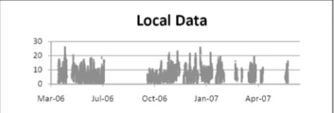
Fig. 1 Met-mast dataset split into a training and a test period.

past multiple-year dataset. It is noted that the in-situ data acquired by erecting a tall met-mast at the representative location in terms of meteorological and geographical point of view, where will be developed as a wind farm, is called “site data” while “reference data”

stands for the wind data of nearby weather station.

In this paper, long-term wind data were generated using different MCP methods as well as artificial neural networks. The key issue of the paper is addressed to demonstrate the possibility and quality of prediction using neural network. Thereto this paper compares the prediction accuracy of different MCP models and neural networks for reconstructing long-term wind data with various statistical indices.

As the “site data,” the 70 m-high met-mast measurement at Waljeong New & Renewable Energy Center of Korea Institute of Energy Research near the potential location of an offshore wind farm in Jejudo is employed. As for

“reference data,” two weather stations were chosen. To compare the prediction accuracy of each method, various statistical indices like IOA, BIAS, MAE, RMSE and also mean wind speed were used.

Chapter 2 gives backgrounds about the used data, followed by long-term wind data reconstruction in chapter 3. In Chapter 4, the prediction results are compared statistically. At the end of this paper, we drew a short conclusion and a summary of the results.

2. Backgrounds

The “reference data” in the studied time period from the nearby weather stations (KMA184, AWS781) are almost complete. They are recorded as a 10 minutes average value. For reference, KMA184 is the Jejudo weather observation station located in Jeju-si apart about 23 km from Waljeong-ri and AWS781 is the Gujwa automatic weather station apart from 9 km approximately.

Figure 1 shows the “site data” from the 70 m met- mast erected at Waljeong-ri beach, north-eastern region in Jejudo. This data is also recorded as a 10 minutes average, but the data is fragmentary and only available over short intervals as shown in the figure. The data should be split into two datasets, a training dataset and a test dataset, to guarantee a validation with unused dataset. All in all there are over 34000 measuring points available. This is enough for training neural network training and also for testing.

3. Long-Term Correction 3.1 Regression MCP

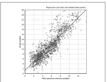
The regression MCP finds meteorological correlation between site data and reference data as a linear or higher order function, whichever fits best between datasets.

In case MCP models embedded in WindPro software

, a linear regression fitting is used to create the long- term data. Because that every traditional MCP model is only possible to use single reference dataset, we created two different predictions, one for each reference dataset;

KMA184 and AWS781. Therefore only wind speed data

from the measurement stations with more than 1 m/s

were used to generate the regression line for the

different wind direction bins (or sectors) as shown in

Figure 2.

Fig. 2 Linear regression of a wind directional bin.

Fig. 3 Trigonometric decomposition of wind vector

Fig. 4 Neural network layer and node design 5-6-1 (8-6-1). WD represents wind direction data, S stands for weather station.

3.2 Matrix MCP

The matrix MCP correlates wind datasets considering each wind direction bins so that N by N correlation matrix is constructed, where N is the number of wind directional bins. If only diagonal terms of the correlation matrix is used, it is the same that the regression MCP model.

Two different predictions were made with the matrix MCP, too. The data is arranged in 10 degree wind direction bins. Wind speeds under 1 m/s were skipped as a calm case.

There are two more MCP models in WindPro software:

the wind index and the Weibull MCP methods. Regarding the relatively poor performance reported by McKenzie et al.

, these models were not used in our study.

3.3 Neural Network

To generate long-term wind data with a neural network, Alyuda NeuroIntelligence software

was employed.

Generally, the more input information to neural network, the better result gets. At the same time, it is also necessary to exclude wrong data like outliers, typhoon period, etc. Contrary to general MCPs, neural

network can accommodate multiple data sets as input, so in this case the data of both stations’ datasets were considered at once.

More over, not only wind speed but also wind direction and clock time information were considered in neural network as a trigonometric function. Note that wind direction and clock time are both cyclic quantity so that

) cos , (sin α α V

V r =

(see the convention in Figure 3).

As for a neural network model, feed forward model and the 5-6-1 (8-6-1) layer & node design shown in Figure 4 were chosen as an optimum.

4. Results and Discussion

In order to investigate the prediction trend visually,

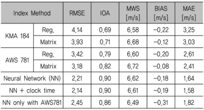
Table 1. Statistical comparison of wind speed predictions by MCP models and neural network. (The best value for the RMSE, BIAS and the MAE would be 0. The best IOA index is 1. The mean wind speed of observation is 6.8 m/s)

Index Method RMSE IOA MWS [m/s]

BIAS [m/s]

MAE [m/s]

KMA 184 Reg. 4.14 0.69 6.58 -0.22 3.25 Matrix 3.93 0.71 6.68 -0.12 3.03

AWS 781 Reg. 3.42 0.79 6.60 -0.20 2.61 Matrix 3.18 0.82 6.72 -0.08 2.41 Neural Network (NN) 2.21 0.90 6.62 -0.18 1.64 NN + clock time 2.14 0.90 6.61 -0.19 1.58 NN only with AWS781 2.45 0.86 6.49 -0.31 1.82

Fig. 5 Scatter plot between the linear regression MCP and KMA184 dataset.

Fig. 6 Result of the Matrix MCP for the AWS781 data.

the predicted wind speed versus the observation is plotted in Figures 5 to 7 and 10. The thick solid lines show the best possible result.

4.1 Regression and Matrix MCP

Both regression and matrix MCPs showed better prediction with AWS781 dataset, the closer reference station, rather than KMA184. As listed in Table 1. BIAS error of matrix MCP, which represents the average deviation of the prediction from the wind speed, has even the best value of all methods.

Figure 5 shows the scatter plot of the prediction with KMA184 dataset by linear regression MCP and the observation, where we can see a wide dispersion.

Figure 6 shows the better agreement between the matrix MCP with KMA781 dataset. As we can see, the dispersion from the best fit line is getting narrower compared to the former case, Figure 5. Also the number of the outliers is fewer. The allocation of the results is constant for all wind speeds.

4.2 Neural Network

Several layer and node designs were tested until finding a best combination. A 5-6-1 design with all input data (wind speed, wind direction of both stations combined with clock time) offers the best prediction.

Hereto Figure 7 shows the predicted wind speed versus the observation.

Comparing the Indices in Table 1, neural network seems to be the best choice for regenerating long-term wind data in our case. However, the distribution of the results of neural network (Figure 7) is much better than the matrix MCP prediction (Figure 6).

By contrast a weakness of neural network is that the

quality of the prediction results varies for different

wind speed ranges. For low wind speed range of the

Fig. 7 MCP prediction of the neural network with 5-6-1 layer and node design.

Fig. 8 Comparison of wind speed time-series between the neural network prediction and the observation.

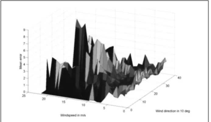
Fig. 9 Prediction error depended of wind speed and wind direction.

Table 2. Contribution of each dataset to long-term prediction

Dataset Contribution

Wind Speed KMA184 5%

Wind Speed AWS781 79%

Wind Direction KMA184 9%

Wind Direction AWS781 5%

Time 2%

observation (less than 2 m/s), the predicted result shows over prediction while under prediction in higher wind speed range. This fact is very important in respect to wind power generation because that wind power is proportional to cubic of wind speed, i.e., P ∝ V

. So for the sensitivity in wind power prediction, accurate prediction in higher wind speed range would be deter- ministic rather than low wind speed range. This trend can be found from BIAS error and that of neural network is quite higher than the others.

In Figure 8, wind speed time-series of the measurement and the prediction are drawn together starting from 13

February 2007 and contains about 1400 data rows. The

graph shows good correspondence but we can find overshooting trend in low wind speed ranges (day 2.5 and 5.7).

To get an overview where prediction error dominates, Figure 9 shows the mean error distribution in dependence of the wind speed and the wind direction.

The biggest error is found between wind speed range of 17 to 22 m/s. In Figure 9, the same trend of Figure 7 is shown, i.e., error increases for higher wind speed.

We get good results with a mean error about 1 m/s for wind speed between 3 to 10 m/s in all wind directions.

For lower wind speed, mean error increases to 3 m/s for all wind directions.

In Table 2 the influence of the individual input data

elements on the output of the best neutral network design

(Figure 7) is shown. Comparing the input influences,

we see that the wind speed at the AWS781 weather

station is the most important for the result. But also

wind directions of both measurement stations have some

influence to the result file and contribution of KMA184

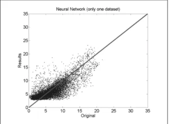
Fig. 10 Result of the Neural Network using data of only one measurement station.

is higher on the contrary. The clock time of the day has only little influence to the result.

For the same condition comparison for neural network and the MCP models, neural network prediction only with single reference dataset was made. The best result was obtained with a 3-11-1 layer and node design (wind speed, wind direction and clock time).

Figure 10 shows the result of this Neural Network with data of only one measurement station. Comparing statistical indices in Table 1, the result of single dataset prediction of neural network shows better result than the traditional MCPs. However, there is again the problem with wind speed range less than 3 m/s.

5. Conclusion

Reliable and accurate methods for regenerating long- term wind data are highly needed in feasibility assessment of wind farm development. This paper shows a possibility of applying neural network for long-term correction of wind data. The results of our research demonstrate that neural network is in the area of aberration very accurate,

like shown in Table 1. The values of MAE, RMSE and IOA are better than those of the traditional MCP methods which are linear regression and matrix MCPs. In a comparison only BIAS error is worse. A weakness of neural network is the unbalanced distribution of the result in wind speed ranges compared to the measure- ment as displayed in Figure 7. This seems to be a problem in the point of evaluation of AEP (Annual Production of Electricity) in wind resource assessment.

Further investigation is to be conducted on this topic.

As good as the results of neural network might look it is always necessary to verify the results.

Acknowledgements

This study was supported by Korea Institute of Energy Research (KIER) and International Association for the Exchange of Students for Technical Experience (IAESTE) Korea KU.

References

[1] EMD, 2008, WindPro v2.6 User Guide.

[2] Morten Lybech Thøgersen, Maurizio Motta Thomas Sørensen & Per Nielsen; Measure-Correlate-Predict Methods, Case Studies and Software Implementation;

EMD Int’l A/S

[3] McKenzie, J., Clive, P., Bulte, H., Chindurzam I., 2008, Considering the Correlate in Measure-Correlate-Predict Techniques, Renewable Energy 2008, Busan BEXCO.

[4] Alyuda, 2007, NeuroIntelligence User Manual and Software.

[5] Madson, H., Kariniotakis, G., Nielsen, H.A., Nielsen, T.S., Pinson, P., 2005, A Protocol for Standardizing the Performance Evaluation of Short-Term Wind Power Prediction Models, Technical University of Denmark.

Franz Vaas 김 현 구

2009년 독일 University of Stuttgart Dipl.-Ing.

(Candidate)

2008년 한국에너지기술연구원 인턴쉽(IAESTE)

1997년 포항공과대학교 기계공학과 공학박사 1998년 미국 아이오와대학교 IIHR 연구원 2000년 포항산업과학연구원 책임연구원 2005년 한국에너지기술연구원 선임연구원

현재 독일 스투트가르트 대학교 기계공학부 대학원 (E-mail : [email protected])

현재 한국에너지기술연구원 풍력발전연구단 (E-mail : [email protected])