Approximating Exact Test of Mutual Independence in Multiway Contingency Tables via Stochastic Approximation Monte Carlo

Approximating Exact Test of Mutual

Independence in Multiway Contingency Tables via Stochastic Approximation Monte Carlo

Sooyoung Cheon

1

Department of Informational Statistics, Korea University

(Received August 16, 2012; Revised September 16, 2012; Accepted October 9, 2012)

Abstract

Monte Carlo methods have been used in exact inference for contingency tables for a long time; however, they suffer from ergodicity and the ability to achieve a desired proportion of valid tables. In this paper, we apply the stochastic approximation Monte Carlo(SAMC; Liang et al., 2007) algorithm, as an adaptive Markov chain Monte Carlo, to the exact test of mutual independence in a multiway contingency table. The performance of SAMC has been investigated on real datasets compared to with existing Markov chain Monte Carlo methods. The numerical results are in favor of the new method in terms of the quality of estimates.

Keywords: Multi-way contingency table, exact inference, Markov chain Monte Carlo, stochastic approx- imation Monte Carlo.

1. Introduction

Contingency table analysis is generally based on the log-linear model to test the goodness-of-fit of the model or the mutual independence test among factors. In the contingency table, the set of all tables with the observed margins is called a reference set, and each table in the reference set is called a valid table. When the expected cell frequencies are small, the exact tests are preferred such as Fisher’s exact test which requires to enumerate the set of all tables with the observed margins. Complete enumeration of the reference set is often infeasible for large tables. Analytical methods to approximate the distribution of the test statistics for large tables take very little time for computation and so offer a useful alternative in situations where it is impossible to enumerate the reference set completely. The most widely used is the chi-squared limiting distribution for either the Pearson chi-squared statistic(χ

) or the Wilks likelihood-ratio statistic(G

); however, for large tables, the p-value estimate obtained using the chi-squared limiting distribution can differ greatly from exact conditional p-values. Efforts to obtain more accurate normal approximations have been done by McCullagh (1986) and Paul and Deng (2000) with the conditional moments of the likelihood ratio statistic that sometimes produces accurate p-values; however, it is still not satisfactory.

This research was supported by Basic Science Research Program through the National Research Foundation of Korea (NRF) funded by the Ministry of Education, Science and Technology (2011-0015000).

1Assistant Professor, Department of Informational Statistics, Korea University, 2511 Sejong-ro, Sejong-city 339-700, South Korea. E-mail: [email protected]

Monte Carlo methods have been also used in exact inference for contingency tables for a long time.

Monte Carlo methods use samples drawn from the reference set for the independence test; however, it is generally difficult to draw samples from the reference set. Many Monte Carlo methods have been developed to avoid such difficulty. Diaconis and Sturmfels (1998) applied the Markov chain Monte Carlo(MCMC) method that draws valid tables from the reference set directly. Diaconis and Sturmfels (1998) employed the Metropolis-Hastings algorithm(MH; Metropolis et al., 1953;

Hastings, 1970) with a Markov basis of the reference set used as a proposal. The Markov basis refers to a finite set of data swaps that allow any two tables in the reference set to be connected and guarantee the irreducibility of the Markov chain. A Markov basis generally takes a too much longer running time to compute, and in even three-way tables the computation can be difficult (Deloera and Onn, 2006). Caffo and Booth (2001) proposed a MCMC method that did not rely on the Markov basis, which is a MCMC extension of the importance sampling algorithm (Booth and Butler, 1999). It uses a rounded normal candidate to update some randomly selected cells while leaving the unselected cells unchanged; however, this use of the rounded normal candidate can make certain tables practically inaccessible despite its theoretical validity. In this case, the method essentially induces a reducible Markov chain and the resulting estimate for the conditional probability can be biased.

In this paper. we apply the stochastic approximation Monte Carlo(SAMC) algorithm (Liang, et al., 2007) to approximate the exact test of mutual independence in a multiway contingency table.

The self-adjusting nature (explained in Section 3) of SAMC enables it to overcome any barrier of the calculation for exact test of contingency tables. SAMC is able to control the proportion of valid tables to a desired value. The work of SAMC on an enlarged reference set with a known Markov basis can improve the convergence rate of the Markov chain and avoids the requirement for the Markov basis of the original reference set. In addition, SAMC ensures its irreducibility on the reference set by employing a Markov basis of the enlarged reference set as the proposal. The performance of SAMC has been investigated on real datasets compared to existing Markov chain Monte Carlo methods. The numerical results are in favor of the new method in terms of quality of estimates.

The remainder of this paper is organized as follows. Section 2 provides a brief description of exact tests of contingency tables. Section 3 reviews the SAMC algorithm and describe how to apply SAMC to test the independence in multiway contingency tables. In Section 4, we apply the proposed method to several examples. In Section 5, we conclude the paper with a brief discussion.

2. Conditional Inference

In this section, we consider a Poisson log-linear model for a given, for example, three-way table used by Caffo and Booth (2001). Detailed reviews and discussion of conditional inference for categorical data can be found in Agresti (1992, 1999, 2002).

Consider I × J × K contingency table X X X with its cell accounts represented as {X

= x

} for i = 1, . . . , I, j = 1, . . . , J and k = 1, . . . , K. Let f (x x x|µ) denote the joint Poisson probability mass function of the data, given under the null model by

f (x x x |µµµ) =

∏

∏

∏

µ

e

x

! , (2.1)

where µ

denotes the expected frequency of the cell (i, j, k), and µ µ µ = (µ

). The saturated model

of expected cell frequencies in log-linear model is usually specified as

log(µ

) = µ + λ

+ λ

+ λ

+ λ

+ λ

+ λ

+ λ

, (2.2) where λ

, λ

and λ

denote a row, column and layer effect, respectively; λ

, λ

and λ

denote respective two-way interaction effects; and λ

denoted the three-way interaction effect.

Let S denote the sufficient set of the model, which is usually the margins. By conditioning on S, the joint mass function (2.1) gives the conditional mass function f (x x x|S) (Caffo and Booth, 2001).

The conditional distribution is usually of the form f (x |S) ∝ 1

∏

i,j,k

x

! , (2.3)

where x x x denotes a three-way contingency table.

Consider a test of the mutual independence model, log(µ

) = µ + λ

+ λ

+ λ

, versus the saturated model corresponding to testing the null hypothesis H

: λ

= λ

= λ

= λ

= 0 for all i, j, k.

The sufficient statistics for λ

, λ

and λ

are the one-dimensional row, column and layer margins, x

, x

and x

, respectively.

Let h be a test statistic for which larger values of h support the alternative hypothesis. For any func- tion h(x x x) where h

= h(x x x

) denotes the value of h at the observed table x x x

, f (x x x) is a probability distribution and I( ·) is an indicator function, it follows that 1/N ∑

t=1

I

(x

) converges to E

(I

(x x x)) almost surely as the sample size N goes to infinite. This provides a Monte Carlo estimate of the exact conditional p-value. As a candidate of h, h(x x x) = −2 [log f(x|ˆµ) − log f(xxx|xxx)]

has been commonly chosen, where ˆ µ µ µ denotes the maximum likelihood estimator of µ µ µ under the null model (Agresti, 2002). The conditional p-value is then defined as

p

= 1 IJ K

∑

∑

∑

I

. (2.4)

3. The SAMC Algorithm for Multiway Tables Analysis

In this section, we briefly review the SAMC (Liang et al., 2007) algorithm and describe how to apply SAMC to test the mutual independence in multiway contingency tables.

3.1. A review of the SAMC algorithm

Suppose that we are working with the following target distribution, f (x) = 1

Z ψ(x x x), x x x ∈ χ, (3.1)

where Z is the normalizing constant, χ is the sample space of x x x, and ψ(x) is a non-negative function.

For contingency tables, χ may correspond to an enlarged reference set, and ψ(x x x) can be defined as in (3.9). Furthermore, we suppose that the sample space has been partitioned according to U (x x x) into m + 1 disjoint subregions: E

= {xxx : U(xxx) ≤ u

}, E

= {xxx : u

< U (x x x) ≤ u

}, . . . , E

= {xxx : u

< U (x x x) ≤ u

}, and E

= {xxx : U(xxx) > u

}. Let θ

= log( ∫

E_i

ψ(x x x)dx x x).

SAMC seeks to draw samples from each of the subregions with a pre-specified frequency. Let x x x

denote a sample drawn from a MH kernel K

(x x x

, · ) with the proposal distribution q(xxx

, · ) and

the stationary distribution

f

(x x x) ∝

m

∑

ψ(x x x) e

I(x x x ∈ E

) + ψ(x x x)I(x ∈ E

), (3.2)

where θ θ θ

= (θ

, . . . , θ

) is a m-vector in a space Θ. For convenience, we set θ

= 0. Here, without loss of generality, we assume that E

is non-empty; that is, ∫

Em

ψ(x x x)dx x x > 0. In practice, E

can be replaced by any subregion that is known to be nonempty. Since χ has been restricted to a compact set by U (x x x), Θ can also be restricted to a compact set. In this paper, we set Θ = [ −10

, 10

]

which is equivalent to setting Θ = R

, as a practical matter.

Let π = (π

, . . . , π

) be a (m + 1)-vector with 0 < π

< 1 and ∑

i=0

π

= 1, which defines desired sampling frequencies for the subregions. Henceforth, π is called the desired sampling distribution.

Define H(θ θ θ

, x x x

) = e

− π, where e

= (e

, . . . , e

) and e

= 1 if x x x

∈ E

and 0 otherwise. Let {γ

} be a positive, non-decreasing sequence satisfying the conditions, (i)

∑

γ

= ∞, (ii)

∑

γ

< ∞, (3.3)

for some δ ∈ (1, 2). In the context of stochastic approximation (Robbins and Monro, 1951), {γ

}

is called the gain factor sequence.

Let J (x x x) denote the index of the subregion that the sample x x x belongs to. Let {K

, s ≥ 0} be a sequence of compact subsets of Θ such that

∪

s≥0

K

= Θ, and K

⊂ int(K

), s ≥ 0, (3.4)

where int(A) denotes the interior of set A. Let χ

be a subset of χ, and let T : χ×Θ → χ

×K

be a measurable function which maps a point in χ × Θ to a random point in χ

× K

. Let σ

denote the number of truncations performed until iteration k. Let B denote the collection of the indices of the subregions from which a sample has been proposed; that is, B contains the indices of all subregions which are known to be non-empty. With above notations, one iteration of SAMC can be described as follows.

The SAMC algorithm:

(a) (Sampling) Simulate a sample x

by a single MH update with the target distribution as defined in (3.2).

(a.1) Generate y y y according to a proposal distribution q(x x x

, y y y). If J (y y y) / ∈ B, set B ← B+{J(yyy)}.

(a.2) Calculate the ratio

r = e

(t)

J (xxx(t) )−θ^(t)_{J (yyy)}

ψ(y y y)q (

y y y, x x x

)

ψ (x x x

) q (

x x x

, y y y

) . (3.5)

(a.3) Accept the proposal with probability min(1, r). If it is accepted, set x x x

= y y y; otherwise, set x x x

= x x x

.

(b) (Weight updating) For all i ∈ B, set θ (

)

i

= θ

+ γ

(

I{

} − π

) − γ

(

I{

} − π

)

. (3.6)

(c) (Varying truncation) If θ θ θ

∈ K

, then set (x x x

, θ θ θ

) = (x x x

, θ θ θ

) and σ

= σ

; otherwise, set (x x x

, θ θ θ

) = T(xxx

, θ θ θ

) and σ

= σ

+ 1.

The self-adjusting mechanism of the SAMC algorithm is obvious: If a proposal is rejected, the weight of the subregion that the current sample belongs to will be adjusted to a larger value, and thus the proposal of jumping out from the current subregion will less likely be rejected in the next iteration. This mechanism warrants that the algorithm will not be trapped by local energy minima.

The SAMC algorithm represents a significant advance in simulations of complex systems for which the energy landscape is rugged.

The proposal distribution q(x x x, y y y) used in the MH updates is required to satisfy the following con- dition: For every x x x ∈ χ, there exist ϵ

> 0 and ϵ

> 0 such that

|xxx − yyy| ≤ ϵ

= ⇒ q(xxx,yyy) ≥ ϵ

, (3.7) where |x − yyy| denotes a certain distance measure between xxx and yyy. This is a natural condition in study of MCMC theory (Roberts and Tweedie, 1996). In practice, this kind of proposals can be easily designed for both discrete and continuum systems as discussed in Liang et al. (2007).

SAMC falls into the category of varying truncation stochastic approximation algorithms (Chen, 2002; Andrieu et al., 2005). Following Liang et al. (2007), we have the following convergence result:

Under the conditions (3.3) and (3.7), for all non-empty subregions, θ

→ C + log

(∫

E_i

ψ(x x x)dx x x )

− log (π

+ υ

) , (3.8)

as t → ∞, where υ

= ∑

j∈{i:Ei=∅}

π

/(m + 1 − m

), m

= # {i : E

= ∅} is the number of empty subregions, and C = − log( ∫

E_m

ψ(x x x)dx x x) + log(π

+ υ

).

Let bπ

= P (x x x

∈ E

) be the probability of sampling from the subregion E

at iteration t.

Equation (3.8) implies that as t → ∞, bπ

will converge to π

+ υ

if E

̸= ∅ and 0 otherwise. With an appropriate specification of π, sampling can be biased to some subregions that are of interest to the user.

3.2. Stochastic approximation Monte Carlo for multiway tables analysis

Now, we describe how to apply SAMC to exact tests of mutual independence on multiway contin- gency tables, and then discuss some practical issues on SAMC implementation.

Let S be the space of constrained tables of sufficient statistics, denoted by S := {xxx : x

= x

, x

= x

, x

= x

}, where x

is an observed dataset. In this paper, we propose to sample from a trial density g(x x x |S), not from f(xxx|S) where xxx ∈ χ, which is defined by

g(x x x|S) ∝ ∏ 1

i,j,k

(x

∨ 0)! , (3.9)

where x

∨ 0 = max(x

, 0). Let U (x x x) = ∑

i,j,k

(x

∧ 0)

where x x x ∈ χ. In that case, SAMC allows the negative entries in multiway tables, and makes an enlarged reference set.

To draw samples from g(x x x|S), SAMC is used as an adaptive Markov chain Monte Carlo. The sample

space is partitioned to ease collection of valid tables according to the function U (x x x) as follows: E

=

{x : U(xxx) = 0}, E

= {xxx : U(xxx) = 1, 2}, E

= {xxx : U(x) = 3, 4}, . . . , E

= {xxx : U(xxx) > 2(m − 1)},

where m is a user-specified number. It is easy to see that the samples in E

are those we want.

Thus the reference set of the table can be represented as Ω = {xxx : U(xxx) = 0} ⊂ χ, and thus χ is called an enlarged set. While the tables in χ\Ω can work as “auxiliary variables” in simulation, which provide connections to different parts of Ω and thus improve the mixing rate of the Markov chain.

In testing for mutual independence, the sufficient statistics are the one-dimensional row, column and layer margins, x

, x

and x

for each i, j and k. To preserve these margins, we propose the following primitive data swap:

1. Randomly draw one element from the set {i, j, k} to determine which to be fixed. Say, i is drawn.

2. Draw i

from the set {1, 2, . . . , I}, draw j

and j

from the set {1, 2, . . . , J} without replacement, and draw k

and k

from the set {1, 2, . . . , K} without replacement.

3. Set y y y = x x x + δδδ, where δδδ denotes an I × J × K table, which has all its elements δ

= 0, apart from δ

= δ

= +1 and δ

= δ

= −1.

4. Accept y y y according to the SAMC rule.

This primitive data swap is the only move that needs to be included in the Markov basis (Dobra, 2003). Thus, the chain induced by the above proposal is irreducible.

Since χ is compact and the proposed primitive data swap proposal satisfies the local positive con- dition given in (3.7), given an appropriate choice of the gain factor sequence {γ

}, we will have the convergence (3.8) holds for the SAMC simulations. Let (x x x

, θ θ θ

), . . . , (x x x

, θ θ θ

) denote the samples drawn by SAMC from the enlarged set χ. Liang (2009) showed that SAMC is actually a dynamic importance sampler and for any integrable function ρ(x x x),

∑

e

(t) J (xxxt)

ρ(x x x

)

∑

e

(t) J (xxxt)

−→ E

ρ(x x x), a.s, (3.10)

as N → ∞, where E

ρ(x x x) denotes the expectation of ρ(x x x) with respect to the target distribution f (x).

Let (y y y

, ν ν ν

), . . . , (y y y

, ν ν ν

) denote the samples drawn from E

= Ω, which form a subset of (x x x

, θ θ θ

), . . . , (x x x

, θ θ θ

). Since g(x x x) is reduced to the target distribution f (x) in (2.3) on E

= Ω, by the convergence result (3.8) ν

t)

converges to a constant almost surely as the number of iteration becomes large, and this implies that the conditional p-value in (2.4) can be estimated by

ˆ p

= 1

n

∑

I(

), (3.11)

where the table y y y

= (y

) in terms of entries. It follows from (3.10), the standard theory of importance sampling that ˆ p

→ p

almost surely as n → ∞.

In the multiway contingency table analysis, we consider several issues for an effective implementation of SAMC.

• Choice of the desired sampling distribution π: According to our aim to draw samples from

E

= Ω, we choose π to bias sampling to the reference set. In this paper, we set π

∝

1/(i + 1)

, i = 0, . . . , m in all simulations. For example, if we set m = 3, then (π

, π

, π

, π

) =

(0.702, 0.176, 0.078, 0.044), which leads to a reasonable high proportion of valid tables.

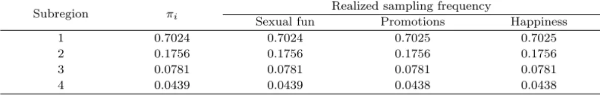
Table 4.1. Comparison of the desired sampling frequencies (π_i, i = 0, . . . , 3) with the realized sampling frequencies for three examples: sexual fun study, promotions study, happiness study.

Subregion πi

Realized sampling frequency

Sexual fun Promotions Happiness

1 0.7024 0.7024 0.7025 0.7025

2 0.1756 0.1756 0.1756 0.1756

3 0.0781 0.0781 0.0781 0.0781

4 0.0439 0.0439 0.0438 0.0438

• Choice of the gain factor sequence and the total number of iterations: To meet condition (3.3), we suggest

γ

=

( T

max(T

, t) )

, t = 0, 1, 2, . . . (3.12)

for pre-specified values of T

> 1 and η ∈ (0.5, 1]. A large value of T

will allow the sampler to reach all subregions rapidly, even for a large system. The appropriateness of the choice of T

and N can be diagnosed by checking the convergence of multiple runs (starting with different points) via an examination for the variation of b θ or π, where b b θ and π denote the estimates of θ and π, b respectively, obtained at the end of a run. If the simulation is diagnosed as unconverged, SAMC should be re-run with a larger value of T

, a larger number of iterations, or both. In this paper, we set η = 1.0 in all simulations.

4. Numerical Examples

In this section, we illustrate the performance of SAMC on three examples for the exact test of mutual independence in multiway contingency tables. SAMC is compared with CaB (the MCMC method by Caffo and Booth (2001)) and the MH method by Diaconis and Sturmfels (1998). The CaB method has been implemented in the R package exactLoglinT est, where, instead of a rounded normal, a rounded student t-variate has been used to generate candidates to update randomly selected cells.

As stated in Caffo and Booth (2001), this generally improves performance. According to the theory of Diaconis and Sturmfels (1998), the MH method should be ideal for these examples, for which a Markov basis is used as the proposal.

For the SAMC algorithm, the sample space was partitioned into four subregions in all examples;

that is, we set E

= {x : U(x) = 0}, E

= {x : U(x) = 1, 2}, E

= {x : U(x) = 3, 4} and E

= {x : U(x) > 4}. For each example, SAMC was run for five times independently. Each run consisted of 5.5 × 10

iterations with T

= 5000, where the first 5.0 × 10

iterations were discarded for the burn-in process and the remaining iterations were used for inference. Table 4.1 compares the desired sampling frequency (obtained in one run) with the realized sampling frequencies for these examples, which are almost identical to each other for each example. This implies that our simulations have converged and we can achieve a pre-specified proportion (i.e., 70.24%) of valid tables in each run.

For comparison, MH was also run for five times independently with 5.5 × 10

iterations including

the first 5.0 × 10

iterations for burn-in process. CaB was also applied to these examples, and each

was run for five times with 5.0 × 10

iterations.

Table 4.2. Comparison of SAMC with the existing CaB (Caffo and Booth, 2001) and MH (Diaconis and Sturmfels, 1998) methods for the sexual fun study example. RMSE: root of mean squared errors of ˆp_h, which was calculated based on five independent runs; Proportion: average proportion of valid tables and its standard deviation (given in parentheses), which was calculated based on five independent runs; CPU: CPU time in minutes cost by a single run on a 3.0GHz personal computer.

Method p-value RMSE Proportion CPU(m)

Exact 0.1137

CaB 0.1131 1.02× 10⁻³ 0.58 (4.10× 10⁻⁴) 28.27

MH 0.1134 6.68× 10⁻⁴ 1.00 1.20

SAMC 0.1137 2.66× 10⁻⁴ 0.70 1.18

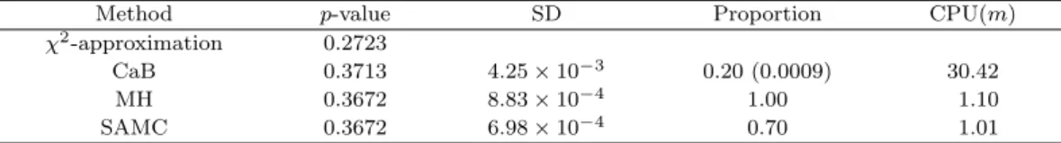
Table 4.3. Comparison of SAMC with CaB and MH for the promotions study example. SD: standard deviation of ˆph, which was calculated based on five independent runs.

Method p-value SD Proportion CPU(m)

χ²-approximation 0.2723

CaB 0.3713 4.25× 10⁻³ 0.20 (0.0009) 30.42

MH 0.3672 8.83× 10⁻⁴ 1.00 1.10

SAMC 0.3672 6.98× 10⁻⁴ 0.70 1.01

4.1. Sexual fun study

This example considers a 4 × 4 two-way contingency table with the wife’s rating and the husband’s rating variables of sexual fun to approximate the exact p-value. Caffo and Booth (2001) suggested a MCMC extension of the importance sampling algorithm, using a rounded normal candidate to update randomly chosen cells while leaving the remainder of the table fixed. The data can be found in Caffo and Booth (2001) that classified 91 people according to degree of feeling on sexual fun.

SAMC was first applied to this example. The numerical results are summarized in Table 4.2. The test produced the insignificance in testing the mutual independence among response, alcohol level and tobacco level. For comparison, MH and CaB were also applied to this example. The comparison indicates that for this example, SAMC works slightly better than the MH method; however, the proportion of valid tables generated by SAMC is 0.7. The theory of Diaconis and Sturmfels (1998) states that the MH method should be ideal; however, SAMC still outperforms MH. This implies that sampling from an enlarged set improves the mixing rate of the Markov chain. CaB still works, but its proportion of valid tables is low at 0.57, and the resulting estimate of p

has a high variability.

Since CaB employed expensive procedures to generate candidate tables, it cost longer CPU time than SAMC and MH at each iteration.

4.2. Promotions study

In this section, we consider a larger table presented by Gastwirth (1988) and analyzed by Agresti (1992). The data refers to “whether promoted” and “race”, stratified by “month of promotion consideration”. Our interest is whether there is a mutual independence relationship among the above three factors. The degree of freedom of this model is 7.

Table 4.3 summarizes the results of SAMC, CaB and MH for this test. The results show that three factors are mutually independent of each other at a significant level 5%. The comparison indicates that SAMC works equally well with the MH method, while they both outperform CaB. Although CaB still works, its proportion of valid tables is very low at 0.20 and the resulting estimate of p

has a high variability; in addition, both SAMC and MH cost less CPU time than CaB.

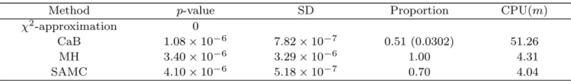
Table 4.4. Comparison of SAMC with CaB and MH for the happiness study example

Method p-value SD Proportion CPU(m)

χ²-approximation 0

CaB 1.08× 10⁻⁶ 7.82× 10⁻⁷ 0.51 (0.0302) 51.26

MH 3.40× 10⁻⁶ 3.29× 10⁻⁶ 1.00 4.31

SAMC 4.10× 10⁻⁶ 5.18× 10⁻⁷ 0.70 4.04

4.3. Happiness study

This example considers the 3 ×4×5 three-way contingency table with the ordering of the happiness, schooling and sibling variables to identify the important bivariate and trivariate moments and identify important location, dispersion and higher order components (Beh and Davy, 1998). The data classifies 1517 people according to their reported happiness, number of completed years of schooling, and number of siblings. Beh and Davy (1997) discussed partitioning the chi-squared statistic for a partially ordered three-way contingency table with a generalized linear model, where happiness is regarded as a response variable and schooling and siblings as the explanatory variables.

The degree of freedom of this model is 50.

All three methods were applied to this example with the same parameter setting as the promotions study. The results were summarized in Table 4.4. At 50 degrees of freedom the test is highly significant and suggest that there is no independence relationship among the happiness, number of years of schooling, and number of siblings for a person. The comparison indicates that SAMC works better than CaB and MH methods. The MH simulation resulted in generating the estimate of p

with a high variability, and CaB has the low proportion of valid tables.

5. Conclusion

In this paper, we have proposed the use of a stochastic approximation Monte Carlo (Liang et al., 2007) algorithm for the exact test of mutual independence in a multiway contingency table.

Since the SAMC sampler can generate a Markov basis by working in an enlarged reference set, the proposed method avoids the reducibility problem that is suffered by existing MCMC methods. The numerical results indicate that the proposed method can outperform existing Monte Carlo methods, such as the MCMC method by Caffo and Booth (2001) and the MH algorithm by Diaconis and Sturmfels (1998).

References

Agresti, A. (1992). A survey of exact inference for contingency tables, Statistical Science, 7, 131–153.

Agresti, A. (1999). Exact inference for categorical data: Recent advances and continuing controversies, Statistics in Medicine, 18, 2191–2207.

Agresti, A. (2002). Categorical Data Analysis, 2nd edition, Wiley.

Andrieu, C., Moulines, ´E. and Priouret, P. (2005). Stability of stochastic approximation under verifiable conditions, SIAM Journal on Control and Optimization, 44, 283–312.

Beh, E. J. and Davy, P. J. (1997). Multiple correspondence analysis of ordinal multi-way contingency tables using orthogonal polynomials, In preparation.

Beh, E. J. and Davy, P. J. (1998). Partitioning Pearson’s chi-squared statistic for a completely ordered three-way contingency table, Australian and New Zealand Journal of Statistics, 40, 465–477.

Booth, J. G. and Butler, R. W. (1999). An importance sampling algorithm for exact conditional test in log-linear models, Biometrika, 86, 321–332.

Caffo, B. S. and Booth, J. G. (2001). A Markov chain Monte Carlo algorithm for approximating exact conditional probabilities, Journal of Computational and Graphical Statistics, 10, 730–745.

Chen, H. F. (2002). Stochastic Approximation and Its Applications, Kluwer Academic Publishers, Dordrecht.

Deloera, J. A. and Onn, S. (2006). Markov basis of three-way tables are arbitrarily complicated, Journal of Symbolic Computation, 41, 173–181.

Diaconis, P. and Sturmfels, B. (1998). Algebraic algorithms for sampling from conditional distributions, The Annals of Statistics, 26, 363–397.

Dobra, A. (2003). Markov bases for decomposable graphical models, Bernoulli, 9, 1093–1108.

Gastwirth, J. L. (1988). Statistical Reasoning in Law and Public Policy 1, Academic, San Diego.

Hastings, W. K. (1970). Monte Carlo sampling methods using Markov chains and their applications, Biometrika, 57, 97–109.

Liang, F. (2009). On the use of stochastic approximation Monte Carlo for Monte Carlo integration, Statistics

& Probability Letters, 79, 581–587.

Liang, F., Liu, C. and Carroll, R. (2007). Stochastic approximation in Monte Carlo computation, Journal of American Statistical Association, 102, 477, 305–320.

McCullagh, P. (1986). The conditional distribution of goodness-of-fit statistics for discrete data, Journal of the American Statistical Association, 81, 104–107.

Metropolis, N., Rosenbluth, A. W., Rosenbluth, M. N., Teller, A. H. and Teller, E. (1953). Equations of state calculations by fast computing machines, Journal of Chemical Physics, 21, 1087–1091.

Paul, S. and Deng, D. (2000). Goodness of fit of generalized linear models to sparse data, Journal of the Royal Statistical Society, Series B, 62, 323–333.

Robbins, H. and Monro, S. (1951). A stochastic approximation method, Annals of Mathematical Statistics, 22, 400–407.

Roberts, G. O. and Tweedie, R. L. (1996). Geometric convergence and central limit theorems for multidi- mensional Hastings and Metropolis algorithms, Biometrika, 83, 95–110.