Spatial Analysis of the Urban Heat Island Using a 3-D City Model

(1)

Spatial Analysis of the Urban Heat Island Using a 3-D City Model

3차원 도시모형을 이용한 도시열섬의 공간분석

전 범 석^* 장 - 미 셀 굴 드 만^**

Bum Seok Chun Jean-Michel Guldmann

요 약 도시열섬 현상은 도심지의 가장 큰 환경문제로 대두되고 있으며, 이는 온도상승, 대기오염, 에너지 수요에 영향을 준다. 이러한 열섬현상에 대하여 많은 건물과 복잡한 공간적/입체적 패턴을 가진 지역의 경우에는 3차원 분석이 전적으로 수행되어야 한다. 본 연구는 2차원자료와 3차원 공간자료를 이 용하여 도시열섬 인자를 파악함에 있다. 또한 공간 통계기법을 이용하여 열섬인자들의 공간적 영향력을 추출한다. 따라서, 도시온도의 예측, 3차원 모델의 생성, 도시인자의 추출, 일반회귀모형과 공간회귀모형 의 구축을 통하여 본 연구를 수행한다. 결과적으로 3차원 도시인자와 인접한 공간영향력들이 도시열섬 현상에 미치는 효과는 크다는 것을 확인할 수 있다. 이를 바탕으로 도시온도 저감을 위한 정책수립에 방 향을 효과적으로 제시할 수 있을 것이다.

키워드 : 도시열섬, 3차원 도시모델, 공간통계

Abstract There is no doubt that the urban heat island (UHI) is a mounting problem in built-up environments, due to energy retention by the surface materials of dense buildings, leading to increased temperatures, air pollution, and energy consumption. To investigate the UHI, three-dimensional (3-D) information is necessary to analyze complex sites, including dense building clusters. In this research, 3-D building geometry information is combined with two-dimensional (2-D) urban surface information to examine the relationship between urban characteristics and temperature. In addition, this research introduces spatial regression models to account for the spatial spillover effects of urban temperatures, and includes the following steps:

(a) estimating urban temperatures, (b) developing a 3-D city model, (c) generating urban parameters, and (d) conducting statistical analyses using both Ordinary Least-Squares (OLS) and Spatial Regression Models. The results demonstrate that 3-D urban characteristics greatly affect temperatures and that neighborhood effects are critical in explaining temperature variations.

Finally, the implications of the results are discussed, providing guidelines for policies to reduce the UHI.

Keyword: Urban Heat Island, 3-D City Model, Spatial Statistics

*Bumseok Chun, Ph.D. (Corresponding author), City and Regional Planning, The Ohio State University.

E-mail: [email protected]

**Jean-Michel Guldmann, Professor, City and Regional Planning, The Ohio State University.

E-mail: [email protected]

1. Introduction

Construction materials, such as concrete and asphalt, absorb thermal energy during daytime and release it during nighttime, leading to temperatures in urban core areas higher than in sur-

rounding suburban and rural areas. Heat energy stored by complicated urban structures is one of the main reasons of high surface temperatures.

This phenomenon is called the urban heat island (UHI). The UHI adversely impacts urban pop- ulations, by inducing heat stress and health prob-

(2)

lem, and worsening air quality through the formation of tropospheric ozone.

This research aims at improving our under- standing of how urban characteristics influence surface temperatures, using both Geographical Information Systems (GIS) and statistical techniques, and making use of data for the urban core of the city of Columbus, Ohio. To model this relationship, both 2-D and 3-D information is used to represent the complex urban geometric structure of urban centers. Much of the earlier UHI research has used 2-D information, such as land uses delineated with satellite imagery and building ground floor boundaries produced by GIS. In the case of homogeneous land uses, this information may be sufficient to predict surface temperatures with good accuracy[7, 22]. However, 3-D information is necessary to analyze more complex sites, including dense building clusters[32, 34]. Chun and Kim (2010) have developed 3-D city models to investigate the impacts of surface features on urban temperatures, employ- ing LiDAR data and geospatial techniques to generate 3-D urban geometry characteristics.

Although their results demonstrate that stereo- scopic city models help derive valuable urban characteristics, they overlooked neighboring effects, and spatial dependence. This paper expands the previous work by Chun and Kim (2010) by specifying and estimating spatial regression models.

The remainder of the paper is organized as follows. Section 2 consists of a literature review.

Section 3 briefly presents the research area.

Section 4 describes the data used and their processing. Model estimation results are discussed in Section 5. Section 6 concludes and out- lines areas for further research.

2. Literature Review

The UHI is an important environmental issue related to surface temperature differentials created

by urban development. Many cities and some of their suburbs have higher temperatures than their surroundings. In general, urban impervious surfaces absorb solar heat and hold it in the absence of cold air advection, particularly in environments of high-rise buildings and low albedo[39, 36].

This increased thermal capacity induces a difference in the micro-climates of urban and rural areas. In particular, land uses are directly related to surface temperatures, as their characteristics affect the storage and radiation of heat, and its partition into latent elements. Heavy particle con- centrations in industrial sites result in higher ra- diative emissivity of particles that explain the absorption of solar radiation[29]. Similarly, convert- ing soil and vegetation into impervious surfaces is a major cause of the UHI[27]. As a result, much research has focused on how urban temperatures are affected by surface materials.

Vegetative cover decreases the absorption of thermal energy due to evapotranspiration and high albedo. Previous research has found that vegetated areas tend to have lower surface temperatures[1]. Oke (1988) reports that impervious areas have temperatures 2°C higher than those in vegetated districts. Li et al. (2010) show that locations further away from a highway or a metro- politan area are associated with lower surface temperatures. Ca et al. (1998) report that the surface temperatures of a grass field in a park are 19°C lower than those of impervious surfaces.

Landsberg and Maisel (1972) show that impervious materials are obstacles to the emission of thermal energy from ground surfaces by moisture particles, and find that there is a 1~2°C difference between rural and urban areas. Much of the previous research has focused on the influences of urban characteristics on the UHI. Oke (1997) has been among the first to describe a UHI model, using urban geometric patterns. For example, wind speed is reduced by buildings that face each other closely. Weak airflows are one of the factors leading to higher surface temperatures. With

(3)

regard to surface characteristics, the albedo (reflectivity) is also related to the UHI. A high albedo releases thermal energy from the surface, but a low albedo absorbs this energy into the surface[3]. Additionally, thermal storage by surface materials is an important factor in investigating urban energy balances. Most materials used for buildings and impervious surfaces easily store thermal energy. On the other hand, a vegetative cover produces lower surface temperatures, due to much lower absorption of thermal energy resulting from evapotranspiration and high albedo.

For example, the UHI intensity is relatively lower during summer daytime, but it becomes higher during summer nighttime and during all days in winter[21].

Statistical models have been estimated to understand and mitigate the UHI, based upon two types of factors: 2-D surface characteristics and 3-D building infrastructure.

First, land use/cover has long been the 2-D information used in exploring the UHI. Weng (2001), Chen et al. (2006), and Amiri et al. (2009) generate maps displaying land use/cover patterns with images captured by Landsat Thematic Mapper (TM) or ETM+, and analyze the surface temperature characteristics of urban environments.

They find that urban expansion reduces the amount of biomass helping to control surface temperatures. Wilson et al. (2003) explains the UHI with the NDVI calculated from Landsat 7 ETM+ data and GIS land-use data. Their simple linear regression models show that lands covered by impervious materials generate higher surface temperatures. They also explore the relationship between surface temperature, NDVI, and development density. Lower NDVI and higher development density increase surface temperatures.

Similarly, Solecki et al. (2005) concentrate on the NDVI to understand the characteristics of surface temperatures. Most studies focusing on vegetative cover have been performed using the NDVI, which has a negative impact on surface

temperatures.

Second, 3-D building environments generate canyon effects. Built-up environments have relatively lower solar radiation because of the block- ing of sunlight by dense buildings, whereas more sunlight reaches ground surfaces in rural areas.

Despite this difference, surface temperatures in built-up environments are higher than in rural areas, because high-rise buildings trap heat within a limited ground space[36]. Therefore, a 3-D building representation is necessary to understand how urban geometry impacts the UHI[4]. The sky view factor (SVF) and the height-to-width (H/W) ratio are representative measures of these geometric effects[3, 31, 32, 16, 15, 12, 13, 35].

The SVF measures the relationship between visible sky and surrounding structures within a reference circle[31]. It varies between 0 and 1. If an observer cannot see the sky due to buildings and trees obstructions, SVF=0; if the visible sky fills the whole reference circle, SVF=1. Previous research shows that urban temperatures are neg- atively correlated with the SVF[40, 21, 3, 5, 32].

The H/W ratio is another representative measure of street geometry[24, 14, 28]. It impacts surface temperature through airflows. For example, a deep urban canyon (H/W≈10) has high nocturnal temperatures at ground level, as compared to a shallow canyon. A deep urban canyon may create a comfort zone due to shading during daytime, but it does not maintain this comfort at night because of heat accumulation without airflows. The ventilation pattern determined by the H/W ratio has also an impact on surface temperatures. High surface temperatures on impervious surfaces cannot be easily decreased without a low H/W ratio that induces dynamic air circulation. Enough space between buildings plays a role in creating a cooling effect. Offerle et al. (2006) explore the H/W ratio for each land use, considering its mean value for central business districts (CBD), and industrial, residential and rural areas. As expected, the CBD and rural areas have the highest

(4)

and lowest ratios, respectively.

There are several shortcomings that characterize previous research on the UHI. First, much UHI research has relied on 2-D information, such as building footprints, land uses, and census information, while not accounting for real-world 3-D physical elements. It is impossible to investigate complex urban characteristics that influence local climate without 3-D information. However, very little research on the UHI has taken place in the 3-D space because of technical problems.

Second, past research has analyzed the UHI with small sets of variables. For example, Carlson etal.(1981) apply a vegetation index to explain the UHI. Unger etal.(2004) explain UHI intensity with the SVF variable. Kim and Kim (2009) use the HW ratio to analyze microclimate. However, these variables alone are insufficient to describe the UHI because of the diversity of physical and non-physical factors. Third, much previous research has involved statistical analysis with Ordinary Least Squares (OLS) models, excluding spatial effects from adjacent regions. Spatial phenomena often involve spatial dependence, with values observed at one place being related to values at adjacent places. OLS UHI models cannot explain such neighboring effects, and therefore may be biased and misleading. Thus, it ap- pears important to analyze the UHI with both 3-D urban geometry and 2-D information, using spatial statistical models. This is the purpose of this research in a case study of the city of Columbus, Ohio.

3. Research Area

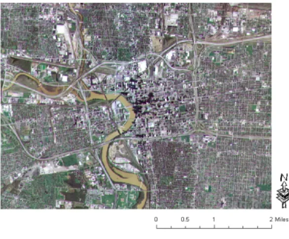
This research focuses on a densely-built section of the City of Columbus, Ohio (Figure 1), with an area of 17.9 square miles (46.5 km2), and including the Central Business District(CBD) , the city’s economic development hub. The Scioto River and the Olentangy River flow from north to south, and merge into one channel near the CBD.

There are parks and recreation places for outdoor activities in the southern part of the research area. The site also includes residential areas. Its temperature has increased by at least 5℃ since 1986. In 2000, the population of the city was 711,470. A continuing population growth since 1950 has induced growth in building construction, leading to increasing surface temperatures.

Fig. 1. Research area

4. Data

The proposed UHI models are based upon three information categories: (1) building information (e.g., building ground floor area, and compactness), (2) 2-D surface information (NDVI, land use, and water stream), and (3) 3-D space information (SVF, Sky View Factor), all extracted from geospatial data, such as LiDAR, Landsat TM, and existing GIS datasets. This section illustrates the implementation of a 3-D city model and the preparation of this information.

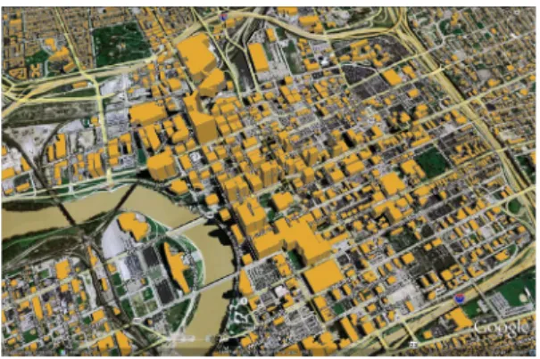
4.1 Three-Dimensional (3-D) City Model A 3-D city model is essential to represent the topology and geometry of built-up environments.

Although much geoinformatic research has focused on detailed building descriptions, our approach delineates box-shaped buildings to investigate the UHI in the 3-D space (Figure 2).

Generating 3-D city models is very time-con-

(5)

suming, and it is difficult to describe building properties (e.g., volume, surface, number of floor, and other characteristics) in terms of exact shapes. We believe that using box-shaped buildings is a good and practical approximation of real building shapes.

Fig. 2. 3-D city model

This research makes use of three geospatial data sources: (1) LiDAR data to estimate each building height, (2) GIS building footprints to describe their ground-level boundaries, and (3) a Digital Terrain Model (DTM) to estimate terrain elevation from sea level. Based upon these datasets, the 3-D city model is developed in two steps: filtering LiDAR data and data integration.

First, filtering LiDAR data by using its properties (e.g., pulse, intensity, and classification) re- moves unnecessary data and reduces the size of the LiDAR dataset. A LiDAR pulse helps detect single and multiple surface layers. Although a tree canopy has multiple layers of leaves and branches, most building roofs are composed of a single layer. From the intensity of a LiDAR pulse, it is possible to distinguish rigid materials from other types of surfaces. The process of filtering the intensity of LiDAR data requires nu- merous trials because intensity values are relative (Faruque, 2003). Pulses with intensity greater than 50 are assumed to detect hard surfaces.

This filtering process helps classify and extract non-ground data, such as building roofs and the

tops of trees.

Second, data integration starts with merging LiDAR data and GIS building footprint that define building boundaries. The spatial joining capability of ArcGIS is used to perform this procedure. We use the highest point among the LiDAR points within each building footprint to specify a pre- liminary height. The actual building height is then computed by excluding the influence of top- ography, using the Digital Elevation Model (DEM).

4.2 Grid Structure

Much past research has used geographically large areas (e.g., nation, state, county, census tract and block) to investigate the relationship between surface temperatures and urban characteristics. Although such data can produce meaningful statistical relationships, they cannot reflect the role of fundamental urban structures, such as buildings, due to the spatial resolution.

Coarse resolutions do not contain detailed building structure data. To examine these characteristics, we need to use a smaller spatial resolution.

A 120m grid structure is used in this research, corresponding to the spatial resolution of the thermal band captured by Landsat TM. Its unit area is smaller than the unit areas used in previous research. Figure 3 illustrates the variations in building volumes captured over this grid.

Superimposing urban characteristics into each grid cell creates the dataset necessary to conduct statistical analyses.

Fig. 3. Building volumes (Unit: 1,000ft^) measured over a 120m grid

(6)

4.3 Dependent Variable: Surface Temperature (AST)

Surface temperatures are derived from the thermal band of Landsat TM captured on July 6, 2007. The Digital number (DN) value of the thermal band varies from 0 to 255, recording the spectral reflectance from the earth surface. This digital number must be numerically converted to a radiometric scale to estimate urban temperatures. The numerical conversion method is provided by the U.S. Geological Survey (USGS) and has been broadly used to map temperatures. Equations (1) and (2) are used to perform this conversion.

Equation (1) is the primary formula to estimate temperature, and includes two calibration constants (_ and _ ) and the spectral radiance at the sensor’s aperture (_). The two constants have been defined by Landsat TM sensors. __is a rescaling factor to predict the original DN value recorded by the initial setting of the sensors. In addition, the National Landsat Archive Production System (NLAPS) provides calibration constants relating _{} and _{} to _ [8]. The equations are as follows:

_{ }





^^

_

 



_

(1)

where T= estimated temperature in Kelvin, _= calibration constant: 1260.56 _= calibration constant: 607.76^ , _= spectral radiance at the sensor’s aperture.

__{}×__{} (2) where _{} ^ _,

_^, ^  ^

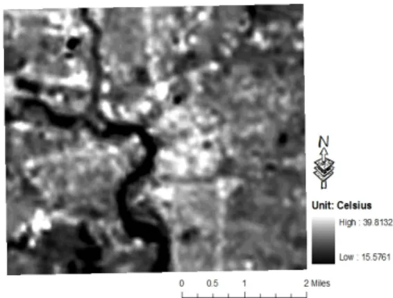
Figure 4 shows the surface temperatures of the study area, as estimated by (1) and (2). The mean temperature is 30.1℃, and the highest temperature 39.8℃. The central part of the study

area, where many buildings are located, has relatively higher temperatures than other places. The two rivers (e.g., the Scioto and the Olentangy) have lower temperatures.

Fig. 4. Surface temperature 4.4.1 Building information

This group includes building ground floor area (BGFA) and compactness (CMPT). BGFA measures the total area of building ground floor in a cell. Each building ground floor is estimated using the appraisal GIS building footprint, with:





  



_ (3)

where ai denotes building I ground floor in a cell, and n represents the number of building footprints in the cell. Figure 5 illustrates building footprints measurements.

_ _

_

(4)

_ __ _ (5)

_ _× _ (6)





  



_ (7)

where  represents the total exterior surface of building i in a cell,  the volume of building i,

_ the compactness of building i, _= the pe- rimeter of building i, = its height, = its

(7)

ground floor area, and n the number of buildings in the cell.

Fig. 5. Building footprint in a cell

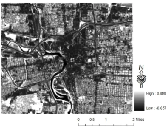
4.4.2 Two-Dimensional(2-D)SurfaceInformation The Normalized Differential Vegetation Index (NDVI) has been extensively used to identify the amount of vegetation coverage. It is computed as a ratio involving different bands reflecting the percentage of vegetative ground cover determined by the amount of plant chlorophyll, in particular, the visible wavelength band (Red: 0.6~0.7) and the Near Infra-Red band (NIR: 0.7~1.1) of Landsat TM, because vegetation has high spectral reflectivity of solar radiation on the NIR band. The NDVI value ranges from -1 to 1.

Values between 0.1 and 1 commonly indicate vegetation coverage. Higher NDVI values indicate healthy vegetation coverage, whereas lower NDVI point to water and impervious materials. Figure 6 illustrates the variations of NDVI over the research area. Light color cells stand for vegetation-covered areas, while dark cells represent non-vegetation areas. The map points to the lack of vegetation in the central district, but also to many vegetated areas around it, corresponding to residential areas and parks.

The primary difference between the urban temperature and NDVI maps is related to spatial resolution. Surface temperatures are based on a 120m pixel size, whereas NDVI is represented by 30m pixels. Therefore, NDVI denotes the total NDVI value in a cell.

Fig. 6. NDVI in the research area

Land Use (LU) is also a basic determinant of the UHI. Land surfaces directly affect heat storage and emission into the air. The relatively higher temperatures in cities as compared to fringe and rural areas result from the diversity of land uses made of diverse materials. The Mid- Ohio Regional Planning Commission (MORPC) has classified land uses into 28 categories, char- acterizing each parcel. In this research, some of these categories have been aggregated, based on similar land properties: Residential, Commercial, Industrial, Open Space, Office, Vacant lots, and Public Service. Non-parcel areas represent roads/streets and water. GIS water surface data from Franklin County Auditor’s database has been added to the grid to measure its impact on temperature. Water covers 3.61% of the research site. Water generally tends to decrease surface temperatures. Although the water area is small, its impact on temperatures can be expected to be significant.

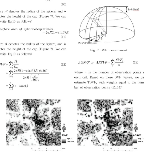
4.4.3 Three-Dimensional (3-D) Space Information This group of variables includes the Sky View Factor (SVF) and solar radiation (ASR). The Sky View Factor (SVF) is numerically defined, as follows (Figure 7)[19]. The solid angle β is the highest vertical angle from the observation point to the building. If we divide the hemisphere into n (=360/φ) pieces, we can define SVF as:

(8)

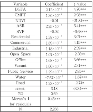
Fig. 8. TSVF and AGSVF values





  



_

_

(8)

where  denotes the portion of visible sky in piece i and  the surface of the hemisphere at piece i. We can define the hemisphere furface and the spherical cap surface as:

  



  



_ ^ (9)

     



  



_  (10) where  denotes the radius of the sphere, and  denotes the height of the cap (Figure 7). We can re-write Eq.10 as follows:

      

     (11) where  denotes the radius of the sphere, and  denotes the height of the cap (Figure 7). We can re-write Eq.10 as follows:





  



_

_





  





^



^





   _





  



   _

(12)

Two measures of SVF are proposed: ground SVF (GSVF) and total SVF (TSVF). GSVF measures SVF at ground level, without any con- sideration of SVF measures on building roofs.

GSVF represents the pedestrian point of view.

Much previous research has concentrated on GSVF. It is difficult to predict GSVF, due to the variety of building locations, shapes, and sizes on limited grounds. Therefore, GSVF is averaged, producing AGSVF (Eq. 13). We similarly estimate the average SVF (ARSVF) at the building roof level:

Fig. 7. SVF measurement

  









_

(13)

where  is the number of observation points in each cell. Based on these SVF values, we can estimate TSVF, with weights equal to the number of observation points (Eq.14):

(9)

 _× _× (14) where  is the number of observation points at ground-level and  the number of observation points at building roof-level. The total number of observation points is 9,152 (7,682 at ground-level, and 1,470 at building roof-level) with a 60m reg- ular interval distance. The values of TSVF and AGSVF over the study area are illustrated in Figure 8.

ASR measures the average solar radiation from the sun. A solar radiation map is generated by the area solar radiation tool in ArcGIS Spatial Analyst extension, requiring the rasterization of the 3D city model and the identification of the latitude of the site.

5. STATISTICAL MODELING

Regression analysis is applied to explore the relationship between the surface temperatures and urban characteristics for the 120m grid. The goal is to find the model that best represents the UHI.

The Ordinary Least Squared (OLS), the Spatial Lag Model (SAR), and the combination of the SAR and SEM models (General Spatial Model:

GSM) are used. New variables are added one by one, in order to avoid multicollinearity¹⁾ problems. Significance and expected signs are considered in this incremental testing.

5.1 OLS Results

This model involves all independent variables without any multicollinearity problem. All the coefficients are statistically significant at the 90%

level using the t-test for each coefficient, and the estimated linear functions explain much of the variability in Log(AST) (R2≈0.69).

1) Multicollinearity takes place when two or more independent variables are highly correlated with each other. It may cause estimation bias. In addition, datasets involving multicollinearity may not produce the inverse matrix necessary for computing the regression coefficients.

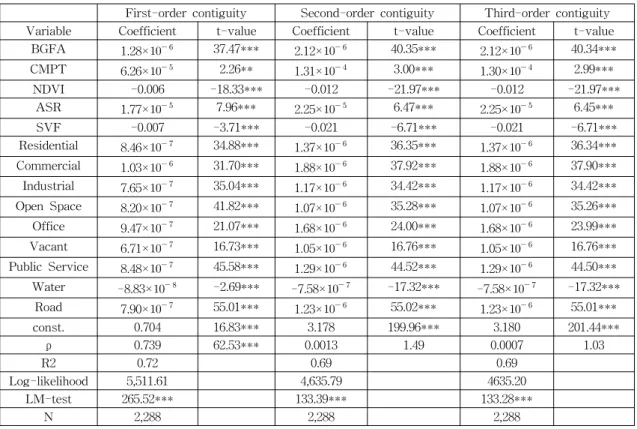
Table 1 indicates positive coefficients for building variables (BGFA and CMPT), solar radiation (ASR), and land-use effects, and negative ones for the sky view factor (SVF), vegetation (NDVI), and water (Water). Thus, an increase in the SVF, NDVI, and Water variables alleviates the UHI, as expected. The negative effect of SVF suggests that the sky view factor at both the ground level and building roofs plays a role in mitigating the UHI. An increase in NDVI induces a decrease in surface temperatures. The soil moisture of green spaces absorbs thermal energy at high surface temperatures, and their energy is then reemitted. Vegetation also plays a critical role in preventing heat exposure because of its shading effects. The water variable, which corre- sponds to the two rivers in the CBD, also reduces surface temperatures.

On the side of the positive effects on the UHI, ASRleads to increased surface temperatures. The amount of absorbed thermal energy into surface materials is the fundamental reason. BGFA pos- itively influences surface temperatures. An increase in BGFA and CMPT leads to higher density, with more impervious surface materials.

Land-use variables also enhance the UHI. For example, the variables Commercial and Office, which represent office and commercial activities, involve parking lots to make access easier. Such impervious surfaces are primary determinants of the UHI. These variables have, by far, the highest regression coefficients. The other land-use variables (Residential, Industrial, Open Space, Office, Vacant, Public Service, and Roa d) have lower, but still positive, coefficients, maybe reflecting the effects of vegetative cover mixed in these land uses.

The Moran’s I indicator is used to assess the spatial autocorrelation of the log-linear model. A value of 0.45 indicates that the spatial autocorrelation among the residuals is significant (Table 1). It is therefore necessary to expand the previous model to reduce the spatial autocorrelation.

(10)

In a first stage, spatial lag models (SAR) are estimated to capture the effects of surface temperatures in neighboring grid cells.

Table 1. Linear regression model results for Log(AST)

Variable Coefficient t-value

BGFA 2.12×^{ } 4.70***

CMPT 1.30×^{ } 2.98***

NDVI -0.01 -21.81***

ASR 2.25×^{ } 6.41***

SVF -0.02 -6.68***

Residential 1.38×^{ } 3.07***

Commercial 1.89×^{ } 4.15***

Industrial 1.18×^{ } 2.59***

Open Space 1.07×^{ } 2.36**

Office 1.68×^{ } 3.66***

Vacant 1.06×^{ } 2.31***

Public Service 1.29×^{ } 2.85**

Water -7.57×^{ } -1.67***

Road 1.23×^{ } 2.74*

const. 3.18 43.34***

R2 0.69

Moran's I for residuals

0.45***

N 2,288

***: Significant at P<0.01; **: Significant at P<0.05;

*: Significant at P<0.1

The Lagrange multiplier (LM) test is used to evaluate the spatial autocorrelation of the residuals. If the LM test still indicates spatial dependency, general spatial models (GSM) are next estimated. Three weight matrices, accounting for first-, second-, and third-order contiguities are considered.

5.2. SAR Results

The SAR models are estimated while considering three different spatial contiguity matrices W:

first-order (8 neighbors), second-order (24 neighbors), and third-order (48 neighbors). The spatial lag coefficient ρ is statistically significant, and with the expected positive sign, only in the first-order contiguity matrix case (0.739), implying that higher temperatures in adjacent cells in-

crease the central cell’s temperature (Table 2).

Also, this SAR model has the highest ^_(0.72), while the ^ of the two other models are very close to the OLS ^. The SAR coefficient esti- mates have the same signs across all three contiguity matrices, and these signs are the same as in the log-linear model (Table 1). Because of these results, only the SAR model with the first-order contiguity matrix is further explored.

Because the LM test is statistically significant, indicating that the error term of the SAR model is still spatially autocorrelated, it is necessary to expand the SAR model into the general spatial model (GSM) models in an effort to further reduce spatial dependency.

5.3. GSM Results

The GSM includes both the spatially correlated error term coefficient λ and the spatial lag term coefficient ρ. The results are presented in Table 3. The coefficients ρ and λ are statistically significant at the 99% level, and, as expected, with positive signs. The R2 of 0.882 represents a 16%

improvement in the model explanatory power, as compared to the SAR model (0.72). The coefficients of all the explanatory variables are significant and with the same signs as the earlier models.

Analyzing the impact of the independent variables in a spatial regression model is different from the approach used in an OLS model, where the partial derivative of the dependent variable with regard to (w.r.t.) an independent variable is commonly used. This derivative can then be in- corporated into the calculation of the elasticity to explore the rate of change of y resulting from a 1% change in x. This simple approach is not val- id when the dependent variable is spatially autocorrelated. The direct, indirect, and total impacts of the independent variables can be measured using the matrix ^ ρ^{ }. The direct impact is related to the impact of variables within the spatial unit itself, without considering any

(11)

First-order contiguity Second-order contiguity Third-order contiguity Variable Coefficient t-value Coefficient t-value Coefficient t-value

BGFA 1.28×^{ } 37.47*** 2.12×^{ } 40.35*** 2.12×^{ } 40.34***

CMPT 6.26×^{ } 2.26** 1.31×^{ } 3.00*** 1.30×^{ } 2.99***

NDVI -0.006 -18.33*** -0.012 -21.97*** -0.012 -21.97***

ASR 1.77×^{ } 7.96*** 2.25×^{ } 6.47*** 2.25×^{ } 6.45***

SVF -0.007 -3.71*** -0.021 -6.71*** -0.021 -6.71***

Residential 8.46×^{ } 34.88*** 1.37×^{ } 36.35*** 1.37×^{ } 36.34***

Commercial 1.03×^{ } 31.70*** 1.88×^{ } 37.92*** 1.88×^{ } 37.90***

Industrial 7.65×^{ } 35.04*** 1.17×^{ } 34.42*** 1.17×^{ } 34.42***

Open Space 8.20×^{ } 41.82*** 1.07×^{ } 35.28*** 1.07×^{ } 35.26***

Office 9.47×^{ } 21.07*** 1.68×^{ } 24.00*** 1.68×^{ } 23.99***

Vacant 6.71×^{ } 16.73*** 1.05×^{ } 16.76*** 1.05×^{ } 16.76***

Public Service 8.48×^{ } 45.58*** 1.29×^{ } 44.52*** 1.29×^{ } 44.50***

Water -8.83×^{ } -2.69*** -7.58×^{ } -17.32*** -7.58×^{ } -17.32***

Road 7.90×^{ } 55.01*** 1.23×^{ } 55.02*** 1.23×^{ } 55.01***

const. 0.704 16.83*** 3.178 199.96*** 3.180 201.44***

ρ 0.739 62.53*** 0.0013 1.49 0.0007 1.03

R2 0.72 0.69 0.69

Log-likelihood 5,511.61 4,635.79 4635.20

LM-test 265.52*** 133.39*** 133.28***

N 2,288 2,288 2,288

***: Significant at P<0.01; **: Significant at P<0.05; *: Significant at P<0.1 Table 2. Spatial lag model results

neighboring effects. The indirect impact represents the effects of the variables inneighboring spatial units, as defined by the contiguity matrix W. Finally, the total impact is the sum of the direct and indirect impacts.

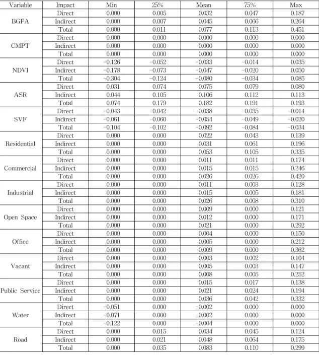
Summary statistics of these impacts, which are computed for each of the 2,288 cells, are presented in Table 4. The mean impact values have signs that are consistent with the signs of the corresponding regression coefficients. All the impacts on surface temperatures of increasing NDVI, SVF, and Water are negative, which is as expected, whereas the other variables have positive impacts on temperatures, implying that the UHI is enhanced. This consistency characterizes all the 2,288 cells for all the variables, except NDVI, which has a positive effect in less than 25% of the cells, most likely in cases of little vegetation. To clearly understand this phenomenon, we need to investigate inter-relationships be-

Table 3. General spatial model results Variable Coefficient t-value

BGFA 1.21×^{ } 34.85***

CMPT 4.76×^{ } 1.80*

NDVI -0.01 -18.78***

ASR 1.29×^{ } 9.95***

SVF -0.01 -3.46***

Residential 8.33×^{ } 28.97***

Commercial 1.06×^{ } 31.46***

Industrial 7.69×^{ } 30.49***

Open Space 7.25×^{ } 28.63***

Office 9.52×^{ } 19.02***

Vacant 6.25×^{ } 12.71***

Public Service 8.24×^{ } 40.23***

Water -3.03×^{ } -8.96***

Road 7.43×^{ } 42.98***

const. 1.159 282.55***

ρ 0.615 282.29***.

λ 0.504 812.45***

R2 0.882

Log-likelihood 5,590.80

***: Significant at P<0.01; **: Significant at P<0.05;

*: Significant at P<0.1

(12)

Variable Impact Min 25% Mean 75% Max

BGFA

Direct 0.000 0.005 0.032 0.047 0.187

Indirect 0.000 0.007 0.045 0.066 0.264

Total 0.000 0.011 0.077 0.113 0.451

CMPT

Direct 0.000 0.000 0.000 0.000 0.000

Indirect 0.000 0.000 0.000 0.000 0.000

Total 0.000 0.000 0.000 0.000 0.000

NDVI

Direct -0.126 -0.052 -0.033 -0.014 0.035

Indirect -0.178 -0.073 -0.047 -0.020 0.050

Total -0.304 -0.124 -0.080 -0.034 0.085

ASR

Direct 0.031 0.074 0.075 0.079 0.080

Indirect 0.044 0.105 0.106 0.112 0.113

Total 0.074 0.179 0.182 0.191 0.193

SVF

Direct -0.043 -0.042 -0.038 -0.035 -0.014

Indirect -0.061 -0.060 -0.054 -0.049 -0.020

Total -0.104 -0.102 -0.092 -0.084 -0.034

Residential

Direct 0.000 0.000 0.022 0.043 0.139

Indirect 0.000 0.000 0.031 0.061 0.196

Total 0.000 0.000 0.053 0.105 0.335

Commercial

Direct 0.000 0.000 0.011 0.011 0.174

Indirect 0.000 0.000 0.015 0.015 0.246

Total 0.000 0.000 0.026 0.026 0.420

Industrial

Direct 0.000 0.000 0.011 0.003 0.128

Indirect 0.000 0.000 0.015 0.005 0.181

Total 0.000 0.000 0.026 0.008 0.310

Open Space

Direct 0.000 0.000 0.009 0.000 0.121

Indirect 0.000 0.000 0.012 0.000 0.171

Total 0.000 0.000 0.021 0.000 0.292

Office

Direct 0.000 0.000 0.004 0.000 0.150

Indirect 0.000 0.000 0.005 0.000 0.212

Total 0.000 0.000 0.009 0.000 0.362

Vacant

Direct 0.000 0.000 0.003 0.002 0.104

Indirect 0.000 0.000 0.005 0.003 0.147

Total 0.000 0.000 0.008 0.005 0.252

Public Service

Direct 0.000 0.000 0.015 0.017 0.138

Indirect 0.000 0.000 0.021 0.024 0.194

Total 0.000 0.000 0.036 0.042 0.332

Water

Direct -0.051 0.000 -0.002 0.000 0.000

Indirect -0.071 0.000 -0.002 0.000 0.000

Total -0.122 0.000 -0.004 0.000 0.000

Road

Direct 0.000 0.015 0.034 0.045 0.124

Indirect 0.000 0.021 0.048 0.064 0.175

Total 0.000 0.035 0.083 0.110 0.299

Table 4. Impact analysis: GSM Model with First-Order Contiguity Matrix

tween variables, using cross-product terms in the regression models. Zero impacts, particularly prevalent for the land-use variables, characterize cells where the impacting variable has a value of zero.

For most of the variables, the indirect impacts are greater than the direct ones, indicating large spillover effects. In addition, the ratio of the di-

rect to indirect impacts is fairly close across cells for any given variables. Ignoring neighboring effects will lead to biases by underestimating the total impacts. For example, the mean total impact (-0.092) of SVF is about 2.5 times greater than the mean direct impact (-0.038), because of the indirect impact (-0.054). In the case of BGFA, the indirect impact (0.045) is 1.4 times greater than

(13)

the direct (0.032). Indirect impacts represent the dominant share of the total impacts, stressing the importance of accounting for neighboring effects.

6. CONCLUSIONS

The primary objective of this research was to develop and implement a modeling methodology for delineating the urban characteristics and factors that enhance or mitigate the UHI. The modeling approach involved different statistical models (OLS and spatial regressions), using 2-D and 3-D urban data generated by satellite, LiDAR, and existing GIS. Earlier research used OLS regression, without accounting for neighboring impacts. However, spatial phenomena are influ- enced by spatial interactions varying with loca- tion and distance. This research has used the spatial lag and the general spatial models to reduce the regression bias resulting from such spatial autocorrelation.

Satellite data were used to estimate surface temperatures and vegetation coverage, and LiDAR data to estimate surface and building elevations.

Available GIS data were used to delineate building boundaries and land uses. These data im- prove over previous research on the UHI by closely approximating the real urban infrastructure and environment in 3-D space. In addition to the application of 3-D city model, this research shows that spatial regressions increase the coefficient of determination by reducing spatial dependency. It indicates that spatial effects should be considered to minimize statistical bias.

However, a first shortcoming of this research is related to the size of the grid cell, 120m, which depends on the spatial resolution of the thermal band by Landsat TM. This size may result in surface information loss. Therefore, further research should use smaller grid scales to identify such information loss. The second shortcoming is related to satellite images captured in July.

Surface temperatures and NDVI vary over the

four seasons. Hence, a temporal analysis of the UHI would clarify the impacts of changing vegetation rates on temperatures. The third shortcoming is the absence of impacts from the anthropogenic heat created by building energy consumption, transportation, and human activity.

However, it is very difficult to obtain detailed data regarding the temporal and spatial variations of anthropogenic heat. Further research could use the statistical data on latent heat sources.

Urban planners and designers play an important role in controlling the building and urban characteristics that influence the UHI. They should enhance smart growth strategies to reduce surface temperatures. They need to increase environmental protection based upon regional com- munity characteristics. Robust UHI models may help simulate the environmental impacts due to proposed changes in urban infrastructures.

Finally, this research is expected to be trans- ferable to South Korea, because the Columbus, Ohio, area is geographically and topographically similar to Seoul.

References

[ 1 ] B. Ackermann, 1987, “Climatology of Chicago area urban rural differences in humidity,”

Theoretical and Applied Climatology, Vol. 26, pp. 427-430.

[ 2 ] R. Amiri, Q. Weng, A. Alimohammadi, and S.

Alavipanah, 2009, “Sparial-temporal dynamics of land surface temperature in relation to frac- tional vegetation cover and land use/cover in the Tabriz urban area, Iran,” Remote Sensing of Environment, Vol. 113, pp. 2606-2617.

[ 3 ] B. Atkinson, 2003, “Numerical modeling of urban heat-island intensity,” Boundary-Layer Meteorology, Vol. 109, pp. 285-310.

[ 4 ] A. Arnfield, and C. Grimmond, 1998, “An urban canyon energy budget model and its application to urban storage heat flux modeling,” Energy and Building, Vol. 27, pp. 61-68.

(14)

[ 5 ] Z. Bottyán, and J. Unger, 2003, “A multiple linear statistical model for estimating the mean maximum urban heat island,” Vol. 75, pp. 233- 243.

[ 6 ] V. Ca, T. Asaeda, and E. Abu, 1998,

“Reductions in air conditioning energy caused by a nearby park,” Energy and Buildings, Vol.

29, pp. 83-92.

[ 7 ] T. Carlson, J. Dodd, S. Benjamin, and J. Cooper, 1981, “Satellite Estimation of the Surface Energy Balance, Moisture Availability and Thermal Inertia,” Journal of Applied Meteorology, Vol. 20, pp. 67-87.

[ 8 ] G. Chander, and B. Markham, 2003, “Revised Landsat-5 TM radiometric calibration proce- dures and postcalibration dynamic ranges,”

IEEE Transactions on Geoscience and Remote Sensing, Vol. 41, no. 11, pp. 2674-2677.

[ 9 ] X. Chen, H. Zhao, P. Li, and Z. Yin, 2006,

“Remote sensing image-based analysis of the relationship between urban heat island and land use/cover changes,” Remote Sensing of Environment, Vol. 104, pp. 133-146.

[10] B. Chun, and H. Kim, 2010, “Analysis of urban heat island effect using information from 3-dimensional city model (3DCM),” Journal of Korea Spatial Information System Society, Vol.

18, no. 4, pp.1-11.

[11] F. Farugue, 2003, “LIDAR Image Processing Creates Useful Imagery,” ArcUser Magazine January-March.

[12] C. Frey, and E. Parlow, 2009, “Geometry effect on the estimation of band reflectance in an urban area,” Theoretical and Applied Climatology, Vol.. 96, pp. 395-406.

[13] T. Gál, F. Lindberge, and J. Unger, 2009,

“Computing continuous sky view factors using 3D urban raster and vector databases: compar- ison and application to urban climate,”

Theoretical and Applied Climatology, Vol. 95, pp. 111-123.

[14] R. Giridharan, S. Ganesan, and S. Lau, 2004,

“Daytime urban heat island effect in high-rise

and high-density residential developments in Hong Kong,” Energy and Buildings, Vol. 36, pp.

525-534.

[15] S. Grimmond, 2007, “Urbanization and global environmental change: local effects of urban warming,” Geographical Journal, Vol. 173, pp.

75-79.

[16] M. Kanda, T. Kawai, and K. Nakagawa, 2005,

“A simple theoretical radiation scheme for regu- lar building arrays,” Boundary-Layer Meteorology, Vol. 114, pp. 71-90.

[17] J. Kim, and D. Kim, 2009, “Effects of a building’s density on flow in urban areas,” Advances in Atmospheric Sciences, Vol. 26, no. 1, pp.

45-56.

[18] H. Landsberg, and T. Maisel, 1972,

“Micrometeorological observations in an area of urban growth,” Boundary-Layer Meteorology, Vol. 2, pp. 365-370.

[19] W. Li, S. PUTRA, P. Yang, 2004, “GIS analysis for the climatic evaluation of 3D urban geometry,” Proceeding of seventh international semi- nar on GIS in developing countries (GISDECO), 10-12 May 2004, Malaysia.

[20] S. Li, Z. Zhao, X. Miaomiao, and Y. Wang, 2010,

“Investigating spatial non-stationary and scale-dependent relationships between urban surface temperature and environmental factors using geographically weighted regression,”

Environmental Modelling & Software, Vol. 25, pp. 1789-1800.

[21] W. Liu, H. You, and J. Dou, 2009, “Urban-rural humidity and temperature differences in the Beijing area,” , Vol. 101, no. 1-2, pp. 237-238.

[22] J. Nichol, 1996, “High-resolution surface temperature patterns related to urban morphology in a tropical city: a satellite based study,”

Journal of Applied Meteorology, Vol. 35, pp.

135-146.

[23] B. Offerle, S. Grimmond, K. Fortuniak, and W.

Pawlak, 2006, “Intraurban differences of surface energy fluxes in a central European city,”

American Meteorological Society, Vol. 45, no. 1,

(15)

pp. 125-136

[24] T. Oke, 1988, “Street design and urban canopy layer climate,”. Energy and Building, Vol. 11, pp. 103-113.

[25] T. Oke, G. Johnson, D. Steyn, and I. Watson, 1991, “Simulation of surface urban heat islands under “Ideal” conditions at night Part 2:

Diagnosis of causation,” Boundary-Layer Meteorology, Vol. 56, pp. 339-358.

[26] T. Oke, 1997, “Urban climates and global environmental change Applied climatology:

Principles and practice,” pp. 273-287, R.D.

Thompson, and A. Perry, eds., Routledge, London.

[27] W. Owen, N. Carlson, and R. Gilles, 1998, “An assessment of satellite remotely sensed land cover parameters in quantitatively describing the climatic effect of urbanization,” International Journal of Remote Sensing, Vol. 19, no. 9, pp.

1663-1681.

[28] C. Ratti, S. Di Sabatino, and R. Britter, 2006,

“Urban texture analysis with image processing techniques: winds and dispersion,” Theoretical and Applied Climatology, Vol. 84: 77-90.

[29] W. Rouse, D. Noad, and J. McCutcheon, 1973,

“Radiation, temperature and atmospheric emis- sivities in a polluted urban atmosphere at Hamilton, Ontario,” Journal of Applied Meteorology, Vol. 12, pp. 798-807.

[30] M. Solecki, C. Rosenzweig, L. Parshall, G. Pope, M. Clark, J. Cox, and M. Wiencke, 2005,

“Mitigation of the heat island effect in urban New Jersey,” Environmental Hazards, Vol. 6, pp. 39-49.

[31] J. Teller, 2003, “A spherical metric for the field-oriented analysis of complex urban open spaces,” Environmental and Planning B:

Planning and Design, Vol. 30, pp. 339-356.

[32] J. Unger, 2004, “Intra-urban relationship between surface geometry and urban heat island:

review and new approach,” Climate Research, Vol. 27, pp. 253-264.

[33] J. Unger, Z. Bottyán, Z, Sümeghy, and Á.

Gulyás, 2004, “Connections between urban heat island and surface parameters: measurements and modeling,” Quarterly Journal of the Hungarian Meteorological Service, Vol. 108, no.

3, pp. 173-194.

[34] J. Unger, 2006, “Modeling of the annual mean maximum urban heat island using 2D and 3D surface parameters,” Climate Research, Vol. 30, pp. 215-226.

[35] J. Unger, 2009, “Connection between urban heat island and sky view factor approximated by a software tool on a 3D urban database,” Internal Journal of Environment and Pollution, Vol. 36, pp. 59-80.

[36] S. Valsson, and A. Bharat, 2009, “Urban heat island: cause for microclimate variations,”

Architecture-Time Space & People, April: pp.

20-25.

[37] Q. Weng, 2001, “A remote sensing-GIS evaluation of urban expansionand its impact on surface temperature in the Zhujiang Delta, China,”

International Journal of Remote Sensing, Vol.

22, no. 10, pp. 1999-2014.

[38] J. Wilson, M. Clay, E. Martin, D. Stuckey, and K. Vedder-Risch, 2003, “Evaluating environmental influences of zoning in urban ecosys- tems with remote sensing,” Remote Sensing of Environment, Vol. 86, pp. 303-321.

[39] O. Wilhelmi, K. Purvis, and R. Harriss, 2004,

“Designing a geospatial information infrastructure for mitigation of heat wave hazards in urban areas,” Natural Hazards Review, Vol. 5, no. 3, pp. 147-158.

[40] S. Yamashita, K. Sekine, M. Shoda, K.

Yamashita, and Y. Hara, 1986, “On relationships between heat-island and sky view factor in the cities of Tama river basin, Japan,” Atmospheric Environment, Vol. 20, pp. 681-686.

[41] 류근원, 김근한, 김혜영, 전철민, 2007, “3차원 GIS 를 활용한 도시소음 시각화에 관한 연구,” 한국공 간정보시스템학회 논문지, 제9권, 제3호, pp. 17-24.

(16)

논문접수 : 2012.01.30

수 정 일 : 1차 2012.06.23 /2차 2012.07.19 심사완료 : 2012.07.25

Bum Seok Chun

2003 Dept. of Geoinformatics, Inha University, S.Korea (B.E.)

2006 Geodetic Science, The Ohio State Univesity (M.S.)

2009 City and Regional Planning, The Ohio State University (M.CRP)

2011 City and Regional Planning, The Ohio State University (Ph.D)

2012-Current Lecturer, The Ohio State University Research Expertise

•Spatial analysis and modeling

•Environmental Impact Analysis