논문 2011-48TC-4-5
모바일 애드혹 네트워크에서 MAC 기반 타임 슬롯 예약을 위한 시간 동기화 알고리즘
( A Time Synchronization Algorithm for a Time-Slot Reservation Based MAC in Mobile Ad-Hoc Networks )
허 웅
*
, 하 우 산*
, 유 강 수**
, 최 재 호*** * ( Ung Heo, Yushan He, Kang Soo You, and Jaeho Choi )
요 약
시간동기화는 모바일 통신 시스템에서 중요한 역할을 한다. 특히, 통신 개체들 사이에 정확한 시분할 기법이 요구될 때, 네 트워크 성능에 영향을 미치는 중요한 요소가 될 수 있다. 본 논문에서는 무선 모바일 애드 혹 네트워크를 위한 새로운 시간 동기화 알고리즘을 제시한다. 본 논문의 주요 목적은 레퍼런스 브로드캐스팅에서 발견된 장점을 활용하여 시간 동기화 패킷의 충돌을 줄이는데 있다. 또한 시간 동기화에 대한 수렴시간을 보장하기 위해 정교한 클럭 갱신 기법을 사용한다. 새롭게 제안한 시간 동기화 알고리즘의 성능을 평가하기 위해 모바일 애드 혹 네트워크에 대한 다양한 시나리오를 구성하고 이를 OPNET으 로 구현하여 실험하였다. 컴퓨터 시뮬레이션 결과, 제안한 기법이 시간 동기화의 정확성과 수렴 시간 등의 측면에서 기존의 TSF 방식보다 좋은 성능을 나타내었다.
Abstract
Time synchronization plays an important role in mobile communication systems, particularly, when an accurate time-division mechanism among the communication entities is required. We present a new time synchronization algorithm for a wireless mobile ad-hoc network assuming that communication link is managed by a time-slot reservation-based medium access control protocol. The central idea is to reduce time synchronization packet collisions by exploiting the advantages found in reference broadcasting. In addition, we adopt a sophisticated clock updating scheme to ensure the time synchronization convergence. To verify the performance of our algorithm, a set of network simulations has been performed under various mobile ad-hoc network scenarios using the OPNET. The results obtained from the simulations show that the proposed method outperforms the conventional TSF method in terms of synchronization accuracy and convergence time.
Keywords : Time synchronization, MANET, Reservation-based MAC, Reference broadcasting, Clock updating
Ⅰ. Introduction
Recently, much attention is drawn to studies in ad-hoc networks and their practical applications.
*
학생회원, 전북대학교
(Chonbuk National University)
**
정회원, 전주대학교, 영상정보신기술연구센터
(Jeonju University).
***
정회원-교신저자, 전북대학교
(Div. of EE, Chonbuk National University).
접수일자: 2010년5월4일, 수정완료일: 2011년4월14일
Many of these applications rely on the use of a time synchronization scheme to provide a common time scale for cooperative work among distributed nodes.
For example, energy saving, involving sleep and wake-up modes of operation, makes use of the proper work of a synchronization scheme to avoid the frequent need for the transmission and reception of information in a neighborhood. On the other hand, we find it interesting that the majority of existing medium access control protocols
[1~3]
supportingmultimedia applications, i.e., voice and video, adopt a slotted time structure where synchronized time-slots are used in order to offer a guaranteed service. For an efficient implementation of such protocols, accurate time synchronization is normally assumed by using the global positioning system on either a centralized node or a cluster tree root. However, GPS has drawbacks. It is less flexible and not available ubiquitously (e.g., under foliage and indoors); and it may not be economically infeasible to implement on every nodes.
Time synchronization algorithms, providing a mechanism to synchronize the local clocks of nodes in a network, have been extensively studied and reported in the literature. The Timing Synchronization Function (TSF) is proposed in the IEEE 802.11 standards
[4]
for the purpose of synchronization in the Independent Basic Service Set (IBSS), an ad hoc network with all nodes in each other’s transmission range. Synchronization is achieved by periodically exchanging time information through beacons containing time stamps. In the TSF, each node sends a beacon periodically at a Target Beacon Transmission Time (TBTT). The typical beacon period is 0.1 second. Upon reception of a beacon, a node adjusts the received time stamp taking into account its physical layer delay. The node updates its clock to the value of the adjusted time stamp using a predefined updating rule.An approximate analysis of the TSF in the IBSS case was first attempted in [5]. This analysis shows that no beacons are transmitted successfully in half of the beacon intervals causing some nodes to become asynchronous. In addition, the low probability of receiving a beacon from the node with a faster clock implies severe asynchronous problems when node clocks drift with respect to one another.
Researchers have also proposed other related methods as adaptive variations of the TSF and their literatures can be found in [5~7]. They all share the basic idea of giving the faster-clock nodes a higher priority to transmit a beacon and to reduce the
beacon transmission frequency of slower-clock nodes.
As a well-known example of existing time synchronization protocols developed for wireless sensor networks, Reference Broadcast Synchronization (RBS) has been proposed in [8].
Differing from widely used sender-receiver synchronization, RBS is based on an approach of receiver-receiver synchronization. RBS leverages the broadcast property inherent in a broadcast-based communication medium; that is, the difference in the reception time for the same broadcast message by the nodes is very small.
In the RBS scheme, nodes periodically send a message to their neighbors using a network’s physical layer broadcast. A reference beacon does not include a time stamp; instead, its time of arrival is used by receiving nodes as a reference point for comparing clocks. The receivers within the communication range of a reference beacon sent by a reference node synchronize with one another rather than with the reference node. The recipients, then, exchange this information among themselves. In this way, they can compute the clock offset with each other.
In addition, the sender can broadcast a number of pulses to improve the precision between the receivers.
Another alternative is to perform a least squares linear regression in a sequence of time offsets. RBS can provide an average synchronization error of
by using 30 broadcasts. The overhead of an additional message exchange consumes the network resource and limits its application in some scenarios.
Our proposed synchronization algorithm requires no assistive system such as a GPS or any other special frequency resource. In addition, there are several other factors making it distinctive and compatible to the commercialized IEEE802.11 standard:
l Time synchronization is achieved by periodically exchanging timing information stamped in a beacon following the same context and packet size as its counterpart in the standardized IEEE
802.11 TSF.
l The logical clock of each node is recursively corrected by adjusting both the clock slope and the clock offset. A better accuracy and a shorter convergence time can be expected.
l A unidirectional clock is adopted as specified in the TSF. In other words, the logical clock of each node moves only forward and never backward or freezes.
l The proposed algorithm can be applied to support real time applications such as voice calls that need stringent frame delay and constant throughput.
The fundamentals and theoretical analyses of the proposed synchronization algorithm were first introduced in [9]. Wen et al. [10] presented the performance of the proposed algorithm in different mobility models and showed its superiority to the TSF in both cases. In this paper, we focus on extending our work to evaluate the resilience of the proposed algorithm under different communication environments.
In the following, Section Ⅱ introduces the clock synchronization algorithm for a mobile ad hoc network in which the wireless medium is shared among the nodes using a time-slot reservation oriented medium access control protocol. In Section
Ⅲ, we present a theoretical analysis of the proposed scheme. In Section Ⅳ, the network simulation model is illustrated in detail. In Section Ⅴ, we describe the performance of the proposed scheme in a mobile ad-hoc network. Finally, we conclude in Section Ⅵ.
Ⅱ. The Proposed Synchronization Algorithm
The proposed synchronization algorithm comprises two phases, i.e., the leading node election and the local clock updating. The leading node election provides a relatively high probability for the node with a faster clock to send out a beacon for synchronization. While the local clock updating synchronizes clocks of all of the nodes in the
network by not only setting the time stamp to equal that of the sender but also by repeatedly adjusting the frequency parameters on each beacon reception so that a faster convergence time can be expected.
1. Models and Assumptions
Here, we introduce the clock model used throughout the paper. We adopt the time process model of the node clock proposed in [11]. Since time jittering has a trivial influence on our synchronization purpose, we neglect the corresponding random process. For the same reason we do not consider timing uncertainties due to environmental conditions.
Using these assumptions, a set of Nnode clock equations is defined as follows:
· (1)
where is the time clock offset of node and
is a proportional coefficient representing the clock slope. On restriction of the hardware clock, the initial value of
is bounded in . The initial time offset is less than .We further assume that the node clock is regarded as a linear function in every beacon period.
Synchronization information for any purpose, i.e., management, security, MAC support, and beacon generation, is taken from the output of this time process. The initial coarse synchronization of the nodes is also assumed before the main algorithm is initiated following the requirement of the IEEE 802.11 standard.
2. Leading Node Election
As specified in [8], the nodes, distributed in the IBSS, can receive a packet from the sending node at the same time. In particular, the propagation delay between any two nodes, around , is assumed to be negligible. We exploit this observation to effectively eliminate the beacon contention problem in the TSF by applying a reference packet based back-off process instead of simply choosing a delay
window before the beacon transmission. The leading node selection process proceeds as follows:
1) At the beginning of each beacon transmission period, from the node that utilized the communication medium last, a reference packet (RP) is sent out with a time stamp from its 2) logical clock
. Note that it does not require anyother information from the sender.
3) Upon receiving the RP, all recipients should record their local time
and calculate the time difference ∆
,which equals
.4) The recipients who have their ∆
less than or equals to 0, meaning their local time is not faster than the sender’s logical clock, give up contention for a beacon transmission.5) The recipient nodes with ∆
become beacon transmission candidates. Before sending out the beacon, they need to wait for a fixed amount of count down time
,which is equal to
∆
, where
is a constant parameter. Note that
is a function of ∆
,meaning that it is different from one node to another node.6) If a beacon arrives before
timer expires, every candidate node cancels its
timer countdown and the pending beacon transmission.7) Otherwise, as soon as
expires, any candidate node transmits a beacon including the RP arriving time
, the time stamp
, and the current logical clock offset value .In the special case that the RP sending node has the fastest clock in the network, it transmits a beacon when its time instant equals
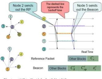
. As an example, consider a set of six nodes in a network running the leading node election depicted in Fig. 1.Assuming to use the medium last, node 2 is in charge of sending out the
. Node 5 wins the election; thus, node 5 sends out the beacon as soon as the
waiting timer expires. The dashed line in그림 1. 선도노드 선출에 대한 예제
Fig. 1. An example of the leading node election.
the figure represents the amount of waiting time for each node. On the other hand, for the case of node 3 and node 4, these nodes do not participate in contention for being the leading node since their clocks are slower than node 1.
Note that the leading node election phase may be failed due to collision of the
. More specifically, when nodes in a cluster are well synchronized, there can be cases where the time difference among node pairs reaches a minimum value so that multiple
may be generated at almost the same time. The
will collide with each other, and then the leading node election failure occurs. However, we argue that the side-effect of such a failure would be negligible. As nodes have already been synchronized to a minimum value, the time synchronization has been achieved. There is no requirement for another synchronization process.2.3 Logical Clock Updating
Upon receiving the beacon, the receiver node records the beacon arriving time
and updates the local logical clock as follows:
╱
(2)
∆(3)
where
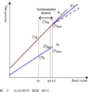
is the time coefficient, and the beacon그림 2. 논리적인 클럭 갱신 Fig. 2. Logical clock updating.
receiving node updates it to
. By updating the time coefficient, Eq. (2) reduces the clock frequency drift and the clock offset at the end of every beacon period. In addition, by taking the influence of the packet delay ∆ into consideration, Eq. (3) pulls the time instant of the receiving node closely up to that of the sender’s clock. The beacon sender’s clock actually slides by the amount of ∆ and becomes
rather than freezes at
by the time the beacon arrives at the receiving node.For a better understanding of the clock updating, consider a pair-wise synchronization procedure illustrated in Fig. 2. In this figure, the horizontal axis indicates the real time, which is indexed an ideal clock . At
the
is received by the beacon sending node with its time stamp
; at the same moment, the time stamp on the receiving node side is recorded and it is
. After a while, the beacon sending node that first runs out of the back-off counter sends out the beacon with the time stamp
. Periodically, the clock synchronization takes
and various processing delay amounts to a small portion of
. Thus,
stands for the time instant of the receiver side at the beacon transmission of the sender; and refers to the time instant of the sender side at the beacon reception ofthe receiver.
From Eq. (3),
is an important value for time stamp updating. Based on the linearity of the clocks, we can easily derive the following set of equations as follows:
(4)
(5)
·
(6)
·
(7)
Combining the above four equations,
(8)
Solving Eq. (8),
(9)
Combining Eq. (8) and (2),
(10)
Applying Eq. (1) at
and combining with Eq.(3) at the receiver side,
·
(11)
By substitution Eq. (9) and (10) into (11),
(12)
Upon receiving the beacon, the parameters
and
are updated by Eq. (10) and (12); and the logical clock of the receiver gets synchronized to that of the sender and the clock frequency drift decreases.Note that all the parameters needed for the calculation are available at the receiver side after
receiving a beacon. As shown in the equations derived, our method distinguishes from those proposed in [6] and [12]. Those conventional ones rely on consecutive beacon receptions from the same reference node for frequency adjustment. Moreover, compared to the TSF, our scheme achieves better accuracy because of the finer adjustment in both the offset and the coefficient parameters. Furthermore, it effectively alleviates the influence of the packet delay components by updating the time instant of the receiver to
rather than the time stamp
provided in the beacon.
Ⅲ. Analysis and Application
In this section, we provide some proofs. First, we prove that nodes with a faster clock have higher probability of being chosen as the leading node to send out the synchronization beacon. As a result, a larger number of nodes in the network can utilize the synchronization information in the beacon rather than waste it because their clocks are faster than the beacon sender’s clock. On the other hand, the second proof indicates that our local clock updating scheme has a small bounded error; hence, this scheme reduces the offset of the clock frequency and ensures a long term clock convergence.
(Lemma 1)
At the end of each leading node election, the node with the fastest clock has the highest priority to send out the beacon.
Proof: In the leading node election phase, every node in the network has a unique back-off time
∆
., Since ∆
, the back-off time
, is closely related to its own logical clock time stamp
on receiving the reference packet.From the viewpoint of the beacon sending node ,
this node sends out the beacon after the expiration of the back-off time
when its logical clock timeinstant equals
. Note that parameter is common to every node, but the parameter
, which is specific to each node. Thus, node actually sets a due for a beacon transmission.Since the initial offset of the logical clock is assumed to be 0, and after every beacon reception, the clock offset is decreased to 0. It is obvious that the node with the greatest clock frequency first has its clock equals
; thus, first this node sends out the beacon.Considering the non-deterministic properties of a wireless network, such as congestion and fading, we can at least safely conclude that nodes with a faster clock have higher probabilities for being chosen as the leading node to send out the synchronization beacon.
(Lemma 2)
The updated clock frequency is upper-bounded by the fastest clock frequency in the field. For each receiving node, it holds that the clock frequency becomes greater after the adjustment
. The frequency offset between the beacon sending nodeand receiving node decreases as
.Proof: Based on the clock updating scheme,
╱
and Lemma 1 prove that
. Thus,
is true.To prove the second inequality, by substituting Eq.
(2) into the above inequality, we obtain:
(13)
After simplification,
(14)
Since the frequency drift is no more than 0.01% in the IEEE 802.11 standard,
is bounded in the range . Thus, the Eq. (14) is true.Combining the two proofs, it is safe to conclude that the local clock updating scheme reduces the drift
그림 3. 시간 분할된 MAC 프로토콜에 대한 예제 Fig. 3. An application to the time-slotted MAC protocol.
of the clock frequency and ensures a long term clock convergence.
Ⅳ. Our Simulation Model
We have conducted a set of simulation by using the OPNET modeler to evaluate the performance of the proposed synchronization scheme. Our simulation model and various simulation configurations are described in this section.
To implement the proposed approach, we developed our own node model. The radio transmitter and receiver modules serve as the interface between packet streams inside a node and the radio link outside the node. The use of a mobility module is to implement the random waypoint (RWP) mobility model, which is commonly used for the mobile nodes in a mobile ad hoc network
[13~15]
. The pause time, distance of each movement step, and boundary, are promoted at the node domain level, thus, can be set directly in the network domain.In the network domain, an arbitrary number of nodes with a transmission range of 200 meters has been randomly deployed in a
500 x 500
meters square area modeling a typical campus network. The IEEE 802.11b specifies that the oscillator counts in increment of with a frequency drift of no more than , The initial value of the time coefficient
is randomly chosen from [0.9999, 1.0001]. All the clocks start asynchronous to one another in the range of .The design parameter
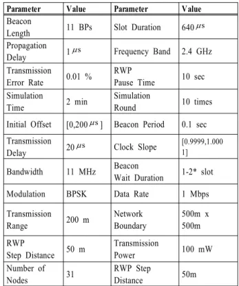
is set to .Attributes and parameters used in our simulation are summarized in Table 1.
Parameter Value Parameter Value
Beacon
Length 11 BPs Slot Duration 640
ms Propagation
Delay 1
ms Frequency Band 2.4 GHz Transmission
Error Rate 0.01 % RWP
Pause Time 10 sec Simulation
Time 2 min Simulation
Round 10 times Initial Offset [0,200
ms ] Beacon Period 0.1 sec Transmission
Delay 20
ms Clock Slope
[0.9999,1.000 1]Bandwidth 11 MHz Beacon
Wait Duration 1-2* slot Modulation BPSK Data Rate 1 Mbps Transmission
Range 200 m Network Boundary
500m x 500m RWP
Step Distance 50 m Transmission
Power 100 mW
Number of
Nodes 31 RWP Step
Distance 50m
표 1. 실험 파라미터
Table 1. Simulation parameters.
V. Simulation Results
After modeling the node and network modules using the OPNET modeler, we move on to evaluate the proposed synchronization method in two scenarios. One is with nodes in a fixed mode scenario and the other in mobile mode scenario. In the case of mobile mode scenario, we assume each mobile node follows the RWP mobility model with a maximum pause time of sec and a maximum step distance of . We have run a set of simulations that are of a two-minute length and collected the maximum time difference between any two clocks on receiving the reference packet at each beacon interval as a performance measurement.
Fig. 4 is the same curve that has been presented in [10]. It shows a comparison between the proposed method and the TSF in terms of the maximum time difference among the nodes when node mobility is disabled. For the proposed clock synchronization scheme, the time difference converges down to
0 2 4 6 8 10 12 14 16 -20
0 20 40 60 80 100 120 140 160 180 200 220
T im e D iff e re n ce ( m s)
Time (seconds) TSF
Proposed Scheme
그림 4. 고정 모드에서 제안된 기법과 TSF의 비교 Fig. 4. Comparison between the proposed scheme and
the TSF for the fixed mode scenario.
0 20 40 60 80 100
0 50 100 150 200 250 300 350 400 450 500 550 600 650 700 750
T im e D iff er e nc e (m s)
Time (seconds) TSF
Proposed Scheme
그림 5. RWP 모드에서 제안된 기법과 TSF 방식의 비 교
Fig. 5. Comparison between the proposed scheme and the TSF in the RWP mobile mode scenario.
after sec, but for the TSF scheme the time difference hardly converges as it bounces around 160 micro-sec.
On the other hand, Fig. 5 shows the performance comparison between the proposed method and the TSF in terms of the maximum time difference among the nodes with the RWP mobility mode enabled. The proposed approach quickly reduces the time difference of the node clocks as the time progresses. The maximum time difference among the nodes converges down to after seconds, however, for the TSF it gets worse and again fails to converge.
In the second phase of the simulation, we have
0 20 40 60 80
0 100 200 300 400 500
T im e D iff e re nc e (m s)
Time(seconds)
rwp90 fix90
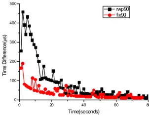
그림 6. SPRR이 0.9일 때 성능 시간차이 Fig. 6. Performance when SPRR is 0.9.
investigated the behavior of our method when the network has the hidden terminal problem. The hidden terminal problem comes from the distributed nature of an ad hoc network and the vulnerable wireless communication environment
[16]
. This network vulnerability leads to packet collision and packet loss.Our interest here is to extend our work to evaluate the resilience of the proposed algorithm in such an unreliable environment.
In this simulation, a new parameter called the successful packet reception rate (SPRR) is included to model the diversified influence of packet reception failure in the wireless ad hoc network.
A higher value of SPRR, i.e., a value nearer to one, refers to a better communication environment. At the beginning of each beacon interval, each node gets assigned with a randomly selected SPRR implying that the impact of unreliable transmission on each node is different from time to time. In other words, we assume that the adverse influence on two consecutive packet receptions is independent from each other. Using two different values of SPRR, i.e., 0.9 and 0.8, we have performed simulations similar to the ones shown in the previous two figures. Fig. 6 shows the performance comparison between the fixed mode and the mobile mode when SPRR is set to 0.9.
The maximum time difference curve for the RWP mobility mode takes somewhat longer time to
0 20 40 60 80 0
100 200 300 400 500 600
T im e D iff er en ce (m s)
Time(seconds)
rwp80 fix80
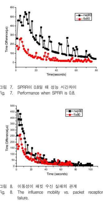
그림 7. SPRR이 0.8일 때 성능 시간차이 Fig. 7. Performance when SPRR is 0.8.
0 20 40 60 80 100
0 50 100 150 200 250 300 350 400 450 500
T im e D iff e re n ce (m s)
Time (seconds) rwp90 fix80
그림 8. 이동성이 패킷 수신 실패의 관계
Fig. 8. The influence mobility vs. packet reception failure.
converge than that of the fixed mode. For both modes, the curves eventually converge down to 15.
Compared to the ideal environment, the increase of the time difference comes from the packet reception failure effect.
Furthermore, Fig. 7 shows the adverse influence of unreliable packet reception when the SPRR gets smaller and equals to 0.8. As shown the synchronization process takes more time as the communication environment gets more vulnerable.
The most distinctive impact is the increase in time difference after convergence. Even for the fixed node scenario, the time difference increases to 18; and for the RWP mobile node mode scenario, the time
differences converge down only to 30 after 80 seconds. However, it is worthwhile to note that unlike the proposed method, the TSF scheme never shows any sign of convergence in the clock synchronization curve.
Finally, Fig. 8 illustrates the performance comparison between two cases where the SPRR is set to 0.8 for the fixed mode and 0.9 for the RWP mobile mode. It is interesting to have a coincidence in the two curves. At the initial transition period the time difference between two curves is distinctive due to the difference in mobility, however, the time differential between two curves quickly disappear as the SPRR becomes in effect. For both curves we find that the convergence time is almost the same, around 30 seconds; and the curves converge down to .
VI. Conclusions
In this paper, we have presented a new clock synchronization algorithm for a mobile ad hoc network in which the wireless medium is shared among the nodes using a time-slot reservation oriented medium access control protocol. The central idea of our proposed method is to reduce time synchronization packet collisions by exploiting the advantages found in reference broadcasting. The results obtained from the simulations have shown us that the proposed method outperforms the conventional TSF method in terms of synchronization accuracy and convergence time. Furthermore, we have investigated the behavior of the proposed method and tested the resilience of the synchronization scheme with an ad hoc network undergoing some vulnerability due to a hidden terminal problem. The simulation results also have yielded a successful clock synchronization results.
References
[1] U. Heo and J. Choi, “Isochronous MAC protocol for real-time service support in MANET,” Proc.
저 자 소 개
허 웅
(학생회원)대한전자공학회 논문지 제47권 TC편 제5호 참조
유 강 수
(정회원) 대한전자공학회 논문지 제47권 TC편 제5호 참조최 재 호
(정회원)-교신저자 대한전자공학회 논문지 제47권 TC편 제5호 참조하 우 산
(학생회원) 2010년 중국 남중민족대학전자공학과 졸업 2010년 전북대학교 전자공학부
석사과정
<주관심분야 : 센서 네트워크, 네 트워크 보안>
of ISITC 2007, pp.100-104, Nov. 2007.
[2] S. Jiang et al., “A simple distributed PRMA for MANETs,” IEEE Trans. on. Vehicular Tech., Vol.
51, No. 2, pp. 293-305, March 2002.
[3] J.C. Fang and G.D. Kondylis, “A synchronous, reservation based medium access control protocol for multihop wireless networks,” Proc. of WCNC 2003, pp. 994-998, March 2003.
[4] IEEE Std.802.11. Wireless LAN Medium Access Control (MAC) and Physical Layer (PHY) specification, 1999 edition.
[5] L. Huang and T.H. Lai, “On the scalability of IEEE 802.11 ad hoc networks,” Proc. of Mobihoc, pp.173-182, June 2002.
[6] D. Zhou and T.H. Lai, “A compatible and scalable clock synchronization protocol in IEEE 802.11 ad hoc networks,” Proc. of ICPP 2005, pp.295-302, June 2005.
[7] Dong Zhou and T.H. Lai, “A scalable and adaptive clock synchronization protocol for IEEE 802.11-based multihop ad hoc networks,” Proc. of MASS 2005, pp.1-8, Nov. 2005.
[8] J. E. Elson, L. Girod, and D. Estrin, “Fine-grained network time synchronization using reference broadcasts,” Proc. of OSDI 2002, pp.147-163, Dec.
2002.
[9] Z. Wen, U. Heo, and J. Choi, “A novel synchronization algorithm for IEEE802.11 TDMA ad-hoc network,” Proc. of MASS-LOCAN 2007, pp. 200-205, October 2007.
[10] Z. Wen, U. Heo, K.S. You, and J. Choi,” Accurate MAC clock synchronization technique for real-time service in ad hoc network,” Proc. of ICITA 2008, pp. 200-205, June 2008.
[11] S. Bregni, “Clock stability characterization and measurement in telecommunications,” IEEE Trans.
on Instrumentation and Measurement, Vol.46, No.6, pp.1284-1294, Dec. 1997.
[12] J.P. Sheu, C.M. Chao, and C.W. Sun, “A clock synchronization algorithm for multi-hop wireless ad hoc networks,” Proc. of ICDCS 2004, pp.
574-581, March 2004.
[13] D. Johnson and D. Maltz, “Dynamic source routing in ad hoc wireless networks,” Mobile Computing, Vol. 353, pp. 153-181, Kluwer Academic Publishers, 1996.
[14] C. Bettstetter and C. Wagner, “The spatial node distribution of the random waypoint mobility model,” Proc. of WMAN, Germany, March 2002.
[15] G. Resta and P. Santi, “An analysis of the node spatial distribution of the random waypoint model for Ad Hoc networks,” Proc. of ACM (POMC), pp.
44-50, Toulouse, France, October 2002.
[16] F.A. Tobagi and L. Kleinrock, “Packet switching in radio channels,” IEEE Trans. on Comm. Vol. 23, No. 12, pp. 1417-1433, Dec. 1975.