1. Introduction
The simplest representation of a zero- dimensional event is the use of a single point set, which assigns an event to a single location.
Traditionally developed techniques provide powerful tools to examine various aspects of univariate point pattern at global and local scales
(Besag and Newell, 1991; Boots and Getis, 1988;
Cressie, 1991; Diggle, 1983; Getis and Boots, 1978;
Ripley, 1981; Silverman, 1986; Upton and Fingleton, 1985). However, many geographic processes representing the occurrence of events are complex requiring multiple point sets, for example, population migration patterns, commuting, housing transactions, multiple purpose
* Department of Geography, Center for Urban and Regional Analysis, The Ohio State University, U.S.A.
An Alternative Method for Assessing Local Spatial Association Among Inter-paired Location Events:
Vector Spatial Autocorrelation in Housing Transactions
Gunhak Lee*
Abstract : It is often challenging to evaluate local spatial association among one- dimensional vectors generally representing paired-location events where two points are physically or functionally connected. This is largely because of complex process of such geographic phenomena itself and partially representational complexity. This paper addresses an alternative way to identify spatially autocorrelated paired-location events (or vectors) at a local scale. In doing so, we propose a statistical algorithm combining univariate point pattern analysis for evaluating local clustering of origin-points and similarity measure of corresponding vectors. For practical use of the suggested method, we present an empirical application using transactions data in a local housing market, particularly recorded from 2004 to 2006 in Franklin County, Ohio in the United States. As a result, several locally characterized similar transactions are identified among a set of vectors showing various local moves associated with communities defined.
Keywords : paired-location event, local spatial association, vector autocorrelation, similarity measure, housing market
trips, and information flow. Such processes have a common assumption that an event of a point set is physically or functionally linked to events of other point sets as a one-dimensional representation. In this context, multivariate point pattern analysis is useful technique to describe a number of types of point sets. However, it cannot effectively describe the spatial pattern of linked events between and among places because it assumes distinct location sets generated by independent processes (Lu and Thill, 2003). Multivariate point pattern analysis is an extended version of single point pattern analysis to multiple point sets.
When a point location is linked to another point location, it is referred to as a paired-location event which is a special case of multiple-location events.
Conventional statistical techniques have been suggested to evaluate the spatial association between two point sets or bivariate point pattern (Bailey and Gatrell, 1995; Upton and Fingleton, 1985). Similar to multivariate point pattern analysis, univariate spatial point pattern analysis is replaced in the multivariate case by exploring the spatial dependence of two independent point sets.
However, there is little emphasis on one to one relationship of a particular linkage, called vectors connecting two end points, and the relationship among inter-paired location events (Lu and Thill, 2003).
In this paper, we propose a statistical method to identify local spatial association of inter-paired location events with respect to vector autocorrelation. The suggested algorithm to assess spatial autocorrelation of vectors takes a hybrid form by combining traditional univariate point pattern analysis technique and vector similarity measure. Our approach will be expected to
provide a methodological support in order to examine the spatial correspondence of paired- location events. The remainder of the paper is organized as follows. The next section introduces previous research dealing with vector spatial autocorrelation, particularly focusing on two main papers published by Berglund and Karlström (1999) and Lu and Thill (2003). Then the algorithm for vector autocorrelation is formally described. For practical use of the developed algorithm, we analyze housing transactions data from 2004 to 2006 in Franklin County, Ohio in the United States and identify spatially autocorrelated transactions and their characteristics related to geographic territories. Finally, the paper is concluded with summary.
2. Methodological approaches to vector spatial autocorrelation
Although a term, vector has its origin in physics representing a quantity having both magnitude (e.g., length or distance) and direction, it is naturally represented as a directed line segment in Euclidean n-space, referred to as a geometric vector. From a physical vector perspective, any geometric vectors can be regarded as equal if they have the same magnitude and direction irrespective of end point locations (Johnson et al., 2002). However, relative locations of end points and their closeness are important for analyses of geographic processes. The spatial association among inter-pairs can be conceptualized by vector spatial autocorrelation. When vectors are directed from nearby locations (origin-points) and similar
magnitude and direction measures, they are positively autocorrelated vectors. On the other hand, negative vector autocorrelation indicates that origin-points of vectors are close together but with dissimilar corresponding vectors. Similarly, if vectors start from different origin-points but end at close locations, they are also negatively autocorrelated. For positive vector autocorrelation, the pattern of vectors is spatially clustered.
Some previous studies dealing with the spatial association among inter-paired location events (vectors) can be found in the literature (Oden and Sokal, 1986; Rosenberg, 2000). However, those studies are limited by controlling one aspect of the geometric properties of a vector such as magnitude and direction. That is, directional vector association concerns directional similarity of vectors start from close locations while distance vector correspondence examines only the spatial association of distances of vectors regardless of direction. Therefore, simultaneous consideration of both magnitude and direction have been received little attention for assessing spatial association among inter-paired location events (Lu and Thill,
2003).
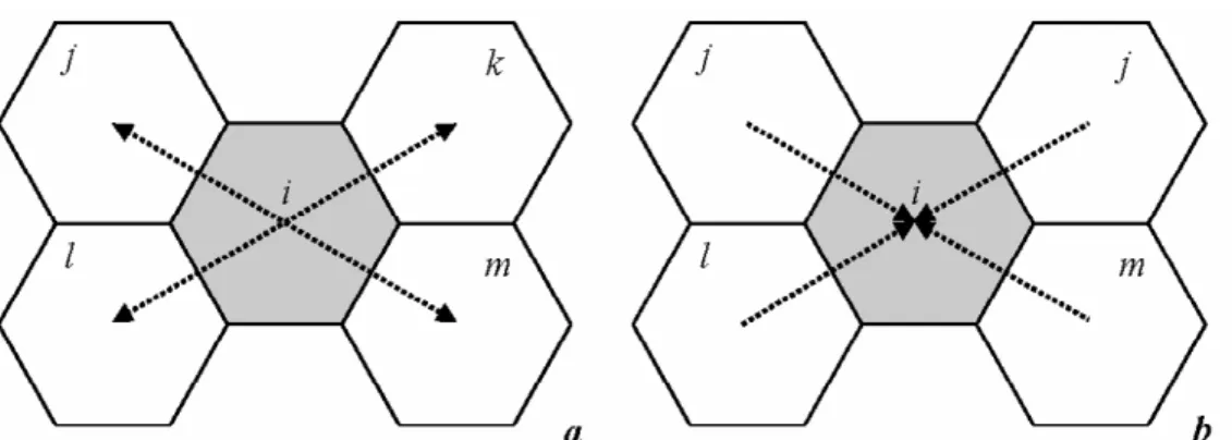
As one of studies utilizing full information of a vector, Berglund and Karlström (1999) is worth noting. They suggested a spatial association statistic Gij(W), where W is a spatial weight matrix of aggregate flows by generalizing the local statistic which was introduced by Getis and Ord (1992) and extended by Ord and Getis (1995). They defined the spatial weight matrices with different metrics such as spatial association of zones and network association of abstract links. Both aspects of association are in fact formally distinguished by Black (1992). In effect, the spatial weight matrices in their paper indicate a binary index of similarity of vectors. Figure 1a illustrates Berglund and Karlström’s definition of the spatial weight matrices with different aspects of a local spatial association for out-flows. By definition of spatial association of zones, vectors ijfi and ilfi are neighbors or similar satisfying the condition that zones j and l are adjacent and starting zone of flow is identical (zone i). Similarly, vectors ikfi and imfl are regarded as similar. Actually, all vectors directed from i are considered as neighbors with definition of network
Figure 1. Spatial weight matrices with two aspects of spatial association a) Out-flows; b) In-flows
association because they are directly interconnected at the same origin i. This spatial association is equivalently applied when zone i is regarded as the same destination of all flows directed from other zones (Figure 1b).
Though they consider both magnitude and direction properties of a vector for identifying local spatial association in flows, this approach may not provide a complete evaluation of vector spatial autocorrelation. For example, even if all neighbored vectors defined by network autocorrelation based on topological relationship are spatially associated, they are not similar in direction as shown in Figure 1. Also, vector patterns of incoming and outgoing flows with different origin or destination within a zone are not addressed (Figure 2a). Notably, evaluating spatial autocorrelation using this approach is essentially sensitive to the size and configuration of zones (Figure 2b).
Alternatively, Lu and Thill (2003) introduced the cluster correspondence between paired-point locations. By examining corresponding clustering of the two sets of end-points (i.e., origin-points
and destination-points), they implicitly deal with the spatial correlation of vectors. That is, they focus on the spatial match between sets of end points of vectors as a proxy of similarity measure among vectors. Although the cluster correspondence they suggested appears to preserve the vector characteristics depicted by distance and direction measures, it may overlook local variation among vectors because it approximates one-dimensional vectors with technically separated two zero- dimensional point sets and then assesses clustering on the basis of averaging spatial proximity. In doing so, this approach takes readily advantage of traditionally well-developed univariate point pattern analysis techniques for an individual point set, while specific information embedded in vectors of paired-location events may not be fully utilized in practice. Moreover, averaging spatial proximity of a set of destination-points1) as a similarity measure among vectors may lose a directional aspect of vectors as the case of Figure 3a. In addition, even if both clusters of origin- points and destination-points identified by any point pattern analytical technique are statistically
Figure 2. Neighbored but not similar vectors
a) With different origins or destinations within a zone; b) Sensitive to zonal definition
significant, actual pattern of vectors may not be spatially autocorrelated or similar due to the different magnitude of vectors leading to different subsequent statistical decision of spatial autocorrelation (Figure 3b).
In summary, it is desirable to keep the original properties of vectors for assessing local spatial autocorrelation of inter-paired location events. The next section suggests an alternative method which brings explicitly the vector characteristics in examining vector autocorrelation.
3. Algorithms for vector autocorrelation
The suggested algorithm in this section is an extended version of Lu and Thill’s approach (2003) by explicitly taking into account the vector properties such as distance and directions, which is referred to as the Algorithm for Vector Autocorrelation-Origin Clustered (AVA-OC). By definition of vector autocorrelation discussed previously, the AVA-OC consists of two main phases: evaluating clustering of origin-points of vectors and measuring similarity of corresponding vectors. Regarding the first step of clustering evaluation, we utilize the count of observations (origin-points) within a neighborhood predefined Figure 3. Incomplete evaluation of vector autocorrelation
a) Different directional vectors; b) Dissimilar vectors in length
and compare it with a well-known Poisson probability distribution for its statistical significance, similar to Lu and Thill, although there are numerous techniques for testing spatial clustering and detecting clusters2). It is known that the probability of the number of events occurring in an area follows a homogeneous Poisson process (Bailey and Gatrell, 1995; Besag and Newell, 1991;
Getis and Boots, 1978). The probability of the number of events, y occurring in an area, A is defined as follows:
fA(y)= e-¬a
where ¬ is an intensity or expected number of events per unit area; a is the area of A.
Then similarity among corresponding vectors to a subset of origin-points is measured by a single similarity measure combining distance and direction, and is tested with a pseudo significance level produced by Monte Carlo simulation approach (Anselin, 1995; Fotheringham and Zhan, 1996). Although a simulation estimate of the theoretical distribution functions under complete spatial randomness (CSR) is computationally intensive, it is useful for statistical inference with unknown distribution properties of statistics (Bailey
and Gatrell, 1995). A theoretical distribution is estimated in general by averaging a number of empirical distributions estimated by repeated independent simulations.
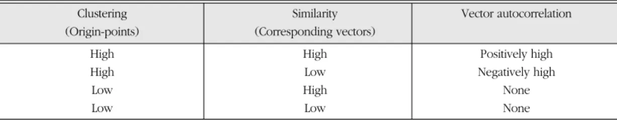
Based on the significance test in each phase, the spatial association of vectors is locally diagnosed with a typology as Table 1.
Consider a paired-location event (vector), denoted by v in a set of vectors V and its neighborhood predefined by a circle centered on its origin point with radius r, denoted by Nvr. In similarity theory, similarity (or more properly dissimilarity) among vectors is typically represented as a distance in metric space (e.g., Euclidean n- space) (Ohbuchi et al., 2002; Santini, 1999). When two variables characterizing vectors (e.g., distance and direction) are concerned, (dis)similarity between two vectors v and w, o|vwcan be defined in a two-dimensional Euclidean space as follows:
where Ωvindicates a direction of a vector v; ‖v‖
is the norm or length of a vector v;
(¬a)y y!
Table 1. Typology of vector autocorrelation
Clustering Similarity Vector autocorrelation
(Origin-points) (Corresponding vectors)
High High Positively high
High Low Negatively high
Low High None
Low Low None
¨ U U U U U o|vw= { }
2
+{ }
Ωv-Ωw 2
RΩ
‖v‖-‖w‖
R∂
R∂= “‖u‖-‖z‖‘- “‖u‖-‖z‖‘ ;
RΩ= “|Ωu-Ωz|‘-max“|Ωu-Ωz|‘ u, z”V
max
u, z”V
max
u, z”V
max
u, z”V
Due to different measurement units, each component is standardized by its range of differences of all pairs of observed vectors (e.g., R∂
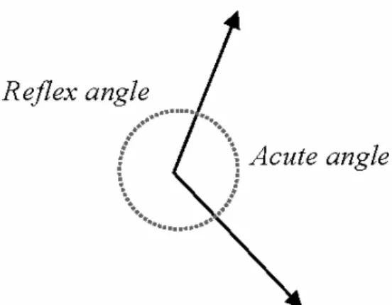
and RΩ). Note that |·| indicates the absolute value of the difference. Computing directional difference of vectors is not straightforward when directions of vectors are conventionally defined as degree angles measured counterclockwise with positive limits [0, 360]. It is noted that as illustrated in Figure 4 directional difference of the two vectors (angle) can be defined as both acute (less than 180°) and reflex angles (greater than 180°and less then 360°), except the zero (0°) and straight angles (180°). Also, note that the sum of both acute and reflex angles generated by two vectors is always 360°. In a general sense, it is reasonable to take a smaller angle (i.e., the acute angle) for directional difference into account. Subsequently, a directional difference of vectors does not exceed 180°as maximum in practice.
However, a special treatment is required for computation to satisfy this constraint, since the directions differ from the number system. For example, the difference between 10°and 350°is arithmetically 340°(in fact, reflex angle) but the
physical difference of degree is 20°(acute angle).
Note that if arithmetic difference is larger than 180°, it represents the reflex angle. Therefore, the following condition ensures the measurement of acute angle for directional difference.
|Ωv-Ωw|=”
Drawn upon the equation structure of (dis)similarity measure, a larger o|vwindicates that two vectors v and w are less similar. The details of the AVA-OC are described as below:
[Evaluation of clustering of the origin-points]
1. For a vector v in V, evaluate clustering among origin-points of vectors within a neighborhood Nvr
with a radius r, centered on the origin- point of vector v with Poisson probability distribution
2. Assign a significance level to a vector v [Evaluation of similarity of corresponding vectors]
3. Identify corresponding lengths and directions of vectors within Nvr
4. Compute an average (dis)similarity measure for all pairs of vectors within Nv
r
5. Extract n random sample vectors in V, where n is the number of vectors in and compute an average (dis)similarity measure for all pairs of n sample vectors
6. Repeat Step 5 for a number of predefined iteration to estimate a simulated probability distribution
7. Evaluate an average (dis)similarity measure for all pairs of vectors within Nvr
with a simulated probability distribution
8. Assign a significance level to a vector v 360-|Ωv-Ωw|if |Ωv-Ωw|>180
|Ωv-Ωw| Otherwise
Figure 4. Directional difference of the two vectors
9. Repeat Step 1-8 until every vector in V is evaluated
4. Empirical application
As an empirical application, we utilize housing property data collected from 2004 to 2006 in Ohio.
This dataset consists of the two subsets of housing transactions in a market: sold house and bought house. Each subset contains geographic information including address, municipality, school district, as well as housing attributes such as sales price, the number of bed and bath rooms, year built, and so on. As preprocess of generating one- dimensional vectors representing paired-location
housing transactions, we filter out the records that seller and buyer are not matched. As a consequence, only matched transactions that a home-seller is identical to the home-buyer are taken into account for analysis.
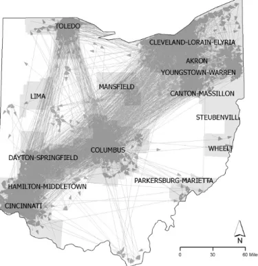
With the matched transaction records, we generate the sets of points, called sold-locations and bought-locations by geocoding addresses of sold and bought houses for each transaction. Then a number of vectors representing housing transactions are generated by linking sold and bought locations, as shown in Figure 5.
From a quick visual inspection, the overall pattern of migration appears prevalent over major metropolitan areas (e.g., Toledo, Columbus, Cincinnati, and Cleveland). Although this is true in some sense, the details are often hidden due to a
Figure 5. Matched housing transactions in Ohio
large number of line segments for housing transactions, which make individual transactions difficult to be distinguished. In fact, 71.4 percents of a total of 17,240 matched transactions is self- contained movement within a county and 28.6 percent is inter-county migrations. Therefore, it is necessary to investigate the transactions at a local scale to obtain more realistic patterns in a local housing market.
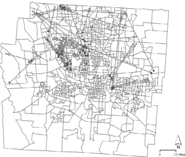
Accordingly, now we focus on the housing transactions within Franklin County, Ohio as a case3). Figure 6 presents all matched transactions (2,066)4)within Franklin County.
From Figure 6, it is hard to identify certain spatial patterns visually. This is what we can expect from paired-location events, particularly when many events are observed in an area and they have various distances and directions.
Therefore, it is desirable to investigate those
phenomena in a formal way. In the next section, we apply the AVA-OC to assess spatial dependence of complex vectors and then identify locally autocorrelated vectors.
5. Assessing local spatial association among housing transactions
For evaluating local clustering of origin-points (e.g., sold-locations) of a transaction, we define the neighborhood (Nv
r) from a circle with a predefined radius r, which is centered on the sold-location of a focused transaction v. Although the number of sold-locations and furthermore the statistical significance of clustering are sensitive to the buffer radius, here we set r to 4,000 feet as an approximation of an average area of blockgroups Figure 6. Matched housing transactions within Franklin County, Ohio
in Franklin County (i.e., 0.6 square miles) for methodological implementation. Note that referring to blockgroups for clustering analysis of sold events might be reasonable because the number of observed sold events within smaller neighborhood (e.g., census block) is fewer and then is insufficient to detect meaningful clusters of inter-vectors. To investigate the effect of neighborhood definition precisely, more systematic sensitivity analysis is needed. Given a neighborhood for a focused transaction, clustering of sold-locations is tested by comparing the number of sold-locations within a neighborhood with a theoretical Poisson probability distribution. On the other hand, the significance of an average dissimilarity of corresponding vectors of sold-locations in a neighborhood is compared with a theoretical probability distribution of an average dissimilarity generated by Monte Carlo simulation of 1,000 iterations (q).
As a final outcome, statistical significance of vector autocorrelation is assessed with respect to Table 1. If clustering of sold-locations is significant and an average dissimilarity of corresponding vectors is significantly less than the average dissimilarity from a theoretical distribution under random process at the significance level of å¯0.01, those vectors are said to be positively autocorrelated. On the other hand, if sold-locations are significantly clustered and an average dissimilarity of corresponding vectors is larger than the average dissimilarity from a theoretical distribution at the significance level of å¯0.01, negative spatial autocorrelation of vectors exists.
Throughout the entire research, we utilize Geographical Information Systems (GIS) for a series of geo-computations - generating flows from
coordinated paired events, extracting neighbors by buffering, and calculating dissimilarity measure among the vectors based on topological relationship. Monte Carlo approach is also programmed and implemented within a GIS environment.
Figure 7 presents spatially autocorrelated vectors.
Locally, 56 housing transactions out of 2,077 total moves from 2004 to 2006 are identified having similar moves within a neighborhood. These movements are positively autocorrelated. That is, home owners who sold houses at nearby locations move out to close places and then bought new houses. No negatively autocorrelated vectors are found. From a visual inspection, locally identified migrations show various spatial patterns of moves, for example, a relatively short movement implying inner migration within a particular community or longer migration from a community to another.
To investigate more detailed spatial patterns at the community level represented as the school district5), it is useful to categorize the communities into several distinctive types in terms of various levels of residential characteristics including size, school quality, crime rate, income, and so on.
Table 2 describes the community type, its description, and related geographic boundaries (school districts).
As shown in Figure 8 and Table 3, significantly similar migrations appear prevalent between communities of categories II and IV which are well-developed suburbs and Columbus which is the central city. Specifically, the move-out takes place most frequently in Upper Arlington (20) and Columbus (16) districts. On the other hand, about 54 percent of the total move-in transactions occur in Upper Arlington (10), Columbus (10), and
Dublin (10) districts. Accordingly, overall Upper Arlington, Columbus, and Dublin are regarded as critical communities for either origin or destination of locally similar moves. Interestingly, most transactions in Upper Arlington (17) are inner
moves within Upper Arlington, particularly presenting relatively short-distance moves from the central to the northern area. Regarding moves from Columbus, the move-out to suburbs dominates the entire transactions. Particularly long-distance moves Figure 7. Locally autocorrelated housing transactions
(Legend is the same as Figure 6)
Table 2. Community type and related school districts
Category Description* School district
I Columbus
II Bexley, Grandview, Upper Arlington
III Whitehall
IV Dublin, Gahanna-Jefferson, Hilliard, Plain Local,
Westerville, Worthington, Reynoldsburg
V Canal Winchester, Groveport, Hamilton,
Madison, Southwestern Referenced by Bayoh et al., 2006
* Note that this column depicts relative features among categories Central city, lower income, bad school quality, high crime rate
Inner suburb, higher income, excellent school quality, lower crime rate
Inner suburb, lower income, excellent school quality, high crime rate
Outer suburb, higher income, excellent school quality, lower crime rate
Outer suburb, lower income, fair school quality, lower crime rate
Figure 8. Locally autocorrelated housing transactions by community (school district)
Table 3. Frequencies for paired locations of significant vectors by community
Bought locations
Total
Bexley
1 1 0 2 0 1 0 1 0 6
(Cat II) Columbus
0 5 4 0 1 1 3 0 2 16
(Cat I) Dublin
0 0 2 0 0 0 0 1 2 5
(Cat IV) Gahanna-
Jefferson 0 0 0 0 0 0 0 1 0 1
(Cat IV) Hilliard
0 1 1 0 2 0 0 0 0 4
(Cat IV) Upper
Arlington 0 3 0 0 0 0 17 0 0 20
(Cat II) Worthington
0 0 3 0 0 0 0 1 0 4
(Cat IV)
Total 1 10 10 2 3 2 20 4 4 56
Bexley (Cat II)
Columbus (Cat I)
Dublin (Cat IV)
Gahanna- Jefferson
(Cat IV)
Hilliard (Cat IV)
Reynoldsb urg (Cat IV)
Upper Arlington
(Cat II)
Westerville (Cat IV)
Worthington (Cat IV)
Sold locations
to outer suburbs (e.g., category IV) including Dublin, Hilliard, Reynoldsburg, and Worthington are apparent. This pattern might be because of relative advantages over inner suburbs, such as relatively cheaper housing price, property tax, amenity, or other preferences. On the contrary, coming-in moves seem to occur in a short distance from inner suburbs (e.g., Bexley and Upper Arlington). Notably, the move-in patterns occur more frequently than the move-out transactions in Dublin. However, Bexley shows the opposite pattern, which the move-out patterns are dominating. The migration of other communities presents the pattern of similar number of moves-in and out.
6. Conclusion
For analyses of physically or functionally linked events across space, it is essential to understand their spatial representation, for example, paired- locations or one-dimensional vector representation.
Although many useful spatial techniques have been developed previously for univariate point pattern analysis or furthermore multivariate point pattern, one to one relationship particularly focusing on a linkage between two points of multiple sets has received little attention.
Especially, spatial association among inter-paired location events (inter-vectors) has not been addressed with appropriate analytical tools. In this paper, we propose an alternative way to identify local spatial association among one-dimensional vectors with a specific interest in the moves in a local housing market. Our approaches are
expected to provide a methodological support to explore a local spatial trend in a complex configuration of a large number of paired-location events, which one can hardly identify the spatial pattern.
The suggested algorithm to assess spatial autocorrelation of vectors (or simply vector autocorrelation) takes a hybrid form by combining traditional univariate point pattern analysis technique and vector similarity measure. Results reveal that several paired-location events are identified as positively autocorrelated at a local scale showing various local moves in a housing market. In order to characterize housing transactions statistically identified, we particularly focus on communities strongly associated with the spatial patterns of residential movements, among various factors which influence housing transactions significantly. Such locally characterized housing transactions seem to be highly related to communities (school districts) classified as various socio-economic levels. Specifically, similar transactions in a local housing market are mainly presented between well-developed suburbs such as Upper Arlington and Dublin, and the central city (Columbus). Interestingly, a majority of significantly similar transactions identified in the City of Upper Arlington are inner-community moves while that is not significant for the overall frequency pattern among communities.
As a final comment, this research may be parameter-sensitive such as neighborhood definition and statistical significance level. Also, only spatial aspects (e.g., vector properties) are considered to estimate similarity among paired- location events. However, multi-dimensional approach including non-spatial attributes - for
example, sales/purchase price, physical features of houses, and socio-demographic characteristics of home owners - is a possible option to define similarity of housing transactions or more generally vector processes. Nevertheless, this research can be regarded as a stepping stone for assessing vector autocorrelation of further complex one- dimensional processes.
Note
1) Note that the degree of clustering of origin-points is measured by the count of points based on the theoretical distribution.
2) See Clark and Evans, 1954; Diggle, 1983; Moran, 1948 for testing spatial clustering. Murray and Estivill-Castro, 1998; Openshaw et al., 1987; Turnbull et al., 1990;
Yamada and Thill, 2004 present techniques for detecting clusters. For a typology of cluster detection, see Besag and Newell, 1991.
3) Franklin County contains 3,290 transactions total including in-migration from other county (427), out- migration to other county (786), and internal-migration within a county (2,077).
4) 10 out of 2,077 transactions are excluded in practice due to address mismatching for geocoding.
5) Total 17 school districts are encompassed fully or partially within Franklin County boundary (Bayoh et al., 2006).
References
Anselin, L., 1995, “Local indicators of spatial association- LISA,” Geographical Analysis 27, pp.93-115.
Bailey, T. C. and Gatrell, A. C., 1995, Interactive spatial data analysis, Harlow, UK: Prentice Hall.
Bayoh, I., Irwin, E. G. and Haab, T., 2006, “Determinants
of residential location choice: How important are local public goods in attracting homeowners to central city locations?” Journal of Regional Science 46(1), pp.97-120.
Berglund, S. and Karlström, A., 1999, “Identifying local spatial association in flow data,” Journal of Geographical Systems 1, pp.219-236.
Besag, J. and Newell, J., 1991, “The detection of clusters in rare diseases,” Journal of the Royal Statistical Society Series A 154(1), pp.143-155.
Black, W. R., 1992, “Network autocorrelation in transport network and flow systems,” Geographical Analysis 24(3), pp.207-222.
Boots, B. and Getis, A., 1988, Point pattern analysis, Newbury Park, CA: Sage Publications.
Clark, P. J. and Evans, F. C., 1954, “Distance to nearest neighbor as a measure of spatial relationship in population,” Ecology 35, pp.445-453.
Cressie, N. A. C., 1991, Statistics for spatial data, New York: John Wiley.
Diggle, P. J., 1983, Statistical analysis of spatial point patterns, London: Academic Press.
Fotheringham, A. S. and Zhan, F. B., 1996, “A comparison of three exploratory methods for cluster detection in spatial point patterns,” Geographical Analysis 28, pp.200-218.
Getis, A. and Boots, B., 1978, Models of spatial processes:
An approach to the study of point, line, and area patterns, Cambridge: Cambridge University Press.
Getis, A. and Ord, J. K., 1992, “The analysis of spatial association by use of distance statistics,”
Geographical Analysis 24, pp.189-206.
Johnson, L. W., Riess, R. D. and Arnold, J. T., 2002, Introduction to linear algebra Addison Wesley.
Lu, Y. and Thill, J.-C., 2003, “Assessing the cluster correspondence between paired point locations,”
Geographical Analysis 35(4), pp.290-309.
Moran, P. A. P., 1948, “The interpretation of statistical maps,” Journal of the Royal Statistical Society Series B 10(2), pp.243-251.
Murray, A. T. and Estivill-Castro, V., 1998, “Cluster discovery techniques for exploratory spatial data analysis,” International Journal of Geographical Information Science 12(5), pp.431-443.
Oden, N. L. and Sokal, R. R., 1986, “Directional autocorrelation: An extension of spatial correlograms in two dimensions,” Systematic Zoology 35, pp.608-617.
Ohbuchi, R., Otagiri, T., Ibato, M. and Takei, T. 2002, Shape-similarity search of three-dimensional models using parameterized statistics. Paper read at 10th Pacific Conference on Computer Graphics and Applications. pp.265-274
Openshaw, S., Charlton, M., Wymer, C. and Craft, A., 1987, “A Mark I geographical analysis machine for the automated analysis of point data sets,”
International Journal of Geographical Information Systems 1, pp.335-358.
Ord, J. K. and Getis, A., 1995, “Local spatial autocorrelation statistics: Distributional issues and application,” Geographical Analysis 27, pp.286-305.
Ripley, B. D., 1981, Spatial statistics, Chichester: John Wiley.
Rosenberg, M. S., 2000, “The bearing correlogram: A new method of analyzing directional spatial autocorrelation,” Geographical Analysis 32(3), pp.267-278.
Santini, S., 1999, “Similarity measures,” IEEE Transactions on Pattern Analysis and Machine Intelligence 21(9), pp.871-883.
Silverman, B. W., 1986, Density estimation, London:
Chapman and Hall.
Turnbull, B. W., Iwano, E. J., Burnett, W. S., Howe, H. J.
and Clark, L. C., 1990, “Monitoring for clusters of disease: Application to leukemia incidence in upstate New York,” American Journal of Epidemiology 132(1), pp.136-143.
Upton, G. J. G. and Fingleton, B., 1985, Spatial data analysis by example, Chichester: John Wiley.
Yamada, I. and Thill, J.-C., 2004, “Comparison of planar and network K-functions in traffic accident analysis,” Journal of Transport Geography 12, pp.149-158.
Correspondence: Gunhak Lee, Department of Geography, The Ohio State University, 0126 Derby Hall, 154 N. Oval Mall, Columbus, Ohio 43210, U.S.A., phone: +1-614-292-8232, e-mail: gunhlee@
gmail.com
최초투고일 2008년 7월 7일 최종접수일 2008년 9월 11일
쌍대위치 이벤트들의 국지적 공간적 연관성을 평가하기 위한 방법론적 연구:
주택거래의 벡터 공간적 자기상관
이건학*
요약`: 물리적 또는 기능적으로 연결된 두 지점에서 발생하는 이벤트(쌍대위치 이벤트)들 사이의 국지적인 공간적 연관성을 평가하는 것은 쉽지 않다. 그것은 대개 그러한 형태의 지리적 현상들이 가지고 있는 프로세스 자체의 복잡한 특성 때문이지만, 실제 공간 상에 서 재현될 때 매우 복잡하게 얽혀 시각적 패턴을 인식하기 어렵기 때문이기도 하다. 이 논문은 국지적 스케일에서 공간적으로 자기상 관된 쌍대위치 이벤트(또는 벡터)들을 확인하기 위한 대안적 방법을 다루고 있다. 제시된 통계적 알고리즘은 (벡터들의) 시작 포인트들 의 클러스터링을 평가하기 위한 단변량 포인트 패턴 분석과 시작 포인트들에 상응하는 벡터들의 유사성 측정을 혼합하여 개발되었다.
사례 분석은 미국 오하이오주 프랭클린 카운티의 지역 주택시장에서 2004년에서 2006년 동안 이루어진 주택거래 데이터를 사용하 여 이루어졌다. 분석 결과, 국지적으로 특성화될 수 있는, 특히 지역 커뮤니티와 연관된 다양한 이동들을 보여주는 주택거래들을 확인 할 수 있었다.
주요어: 쌍대위치 이벤트, 국지적 공간적 연관성, 벡터 자기상관, 유사성 측정, 주택시장 한국경제지리학회지 제11권 제4호 2007(564~579)
* 미국 오하이오 주립대학교 지리학과, 도시 및 지역 분석 연구소