2013 한국유체기계학회 학술대회 발표 논문, 2013년 11월 27-29일, 제주
◎ Original Paper ISSN (Print): 2287-9706
부유식 수처리시스템용 축류펌프의 성능 및 내부유동
패트릭마크싱*⋅최영도**†
Performance and Internal Flow Characteristics of an Axial Flow Pump for a Floating Type Water Treatment System
Patrick Mark Singh
*, Young-Do Choi
**†1)2)Key Words : Axial Pump(축류펌프), Water treatment system(수처리시스템), Performance(성능), Internal flow(내부유동), Cavitation(캐 비테이션)
ABSTRACT
The development of efficient systems for water quality improvement for water sources such as lakes, dams and reservoirs has become a necessity to provide not only a cleaner and safer water to the urban society, but also to provide a cleaner and safer environment for the aquatic organisms living in lakes, dams and reservoirs. This study concentrates on the outlet design and internal flow analysis of an axial flow pump used in a floating type water treatment system completely powered by renewable energy source. The treatment system is designed to raise water from depths of about 3∼5m up to the water surface where it is naturally mixed with air as it is released back to the reservoir. The outlet of a typical axial flow pump is modified to suit the floating type water mixer. The performance of the axial flow pump is studied by investigating the internal flow of the system. Results show that the change in outlet shape does not alter the performance of the original pump at the maximum efficiency point as long as the cross sectional area of inlet is the same as the outlet. The axial pump for floating type water treatment system has good cavitation performance in the whole flow passage.
1. Introduction
Water stratification in reservoirs and lakes is usually formed because of the difference in the water densities between the upper and lower depths. The deeper water has the higher density. During the winter time when the surface water is frozen, the icy top shields the wind mixing effects and the water underneath becomes relatively stable. Thus the high density water of the lower depth stays on the bottom and does not mix with the upper layer water.
Consequently, the water in the lower layer gradually becomes anoxic because of the inadequate supply of dissolved oxygen, and this in turn deteriorates the living conditions for aquatic organisms(1, 2).
Under anoxic conditions, some pollutants in the sediments will be released into the water and a series of problems may be caused such as colour and odour.
The pH level may decrease and the algae’s multiplication may be accelerated.
There are two solutions to the anoxic condition in deeper layer water due to stratification. One is to
* Graduate School, Department of Mechanical Engineering, Mokpo National University (목포대학교 대학원 기계공학과)
** Department of Mechanical Engineering, Mokpo National University (목포대학교 기계공학과, 신재생에너지기술연구소)
† 교신저자(Corresponding Author), E-mail : [email protected]
Fig. 2 Axial pump models: (a) Original pump model (b) Modified pump model for water treatment system
Parameter Value
Impeller diameter 540 mm
Head 4 m
Flow rate 0.83 m3/s
Rotational speed 720 min-1
Blade number 4
Inlet cross sectional area 0.22 m2 Table 1 Specification of axial pump model types A and B
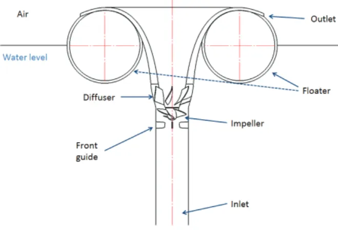
Fig. 1 Schematic view of floating type water treatment system using axial pump
overcome the water stratification. The other is to oxygenate the deep layer water by mixing.
Therefore, to apply the second countermeasure, this study introduces an axial-flow pump system. Axial flow pumps are typically used in high flow rate, low lift applications and can also be submersible(3∼8).
This study investigates the performance and internal flow characteristics of an axial flow pump used in the water treatment system. The system includes a floater which has the simple circular top base. Moreover, as power sources, wind turbine or solar cells can be installed on the top base of the system.
Other methods of water mixing has been discussed by McAliley9 and C ong1. The floating type system is developed because it can be easily applied to suitable locations. As it is not fixed, it can be easily moved to cover wider areas of the lake or reservoir, especially where anoxic conditions are more clearly visible. The use of renewable energy power source also makes the system more environmentally friendly.
2. Axial Pump Model and Numerical Methods
2.1. Floating type water treatment system and axial pump model
Figure 1 illustrates the schematic view of floating type water treatment system using axial pump. The pump is vertically aligned to pump up water from deeper layers. The central part contains the shaft and other mechanical systems. The fluid is pumped through the center and discharged on the sides of the floater, where the water naturally mixes with the atmosphere and goes back to the reservoir. So the top layer goes down as the deeper layer is pumped up and the cycle continues, which oxygenates the water.
Figure 2 shows the axial pump models adopted in this study. As the outlet of the pump installed in the
water treatment system can be modified to find the best suitable shape, the typical pump model (Fig 2(a).
straight type outlet) will be compared by changing the outlet (Fig 2(b). curved type outlet) to suit the floating type water treatment model. The effect of the change in shape will be investigated by studying the internal flow characteristics using numerical analysis. Table 1 presents the design parameters of axial pump model adopted. The design parameters for the pump types A and B are all same but only the outlet shape is different.
2.2. Numerical methods
For the numerical analysis on the pump performance and internal flow, a commercial software of ANSYS CFX(10) is applied. As shown in Fig. 3, a high grid density is required for the impeller surface to achieve reliable CFD calculations.
Fig. 3 Numerical grids of axial-flow pump impeller
Domain Nodes Elements
Inlet & Outlet 4.0×10⁶ 5.3×10⁶
Front Guide Vanes 0.2×10⁶ 1.1×10⁶
Impeller 0.9×10⁶ 3.3×10⁶
Diffuser 0.8×10⁶ 4.3×10⁶
Total (All Domains) 5.9×10⁶ 14.0×10⁶
Table 2 Mesh information
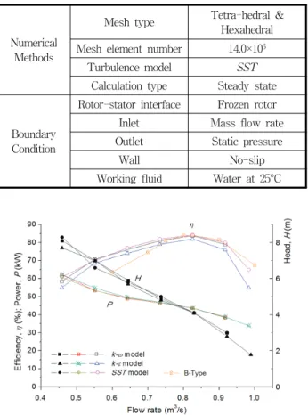
Numerical Methods
Mesh type Tetra-hedral &
Hexahedral Mesh element number 14.0×10⁶
Turbulence model SST
Calculation type Steady state
Boundary Condition
Rotor-stator interface Frozen rotor
Inlet Mass flow rate
Outlet Static pressure
Wall No-slip
Working fluid Water at 25°C Table 3 Boundary conditions and numerical methods
Fig. 4 Turbulence model dependence test of the axial pump model B
The analysis for this study is done by using tetrahedral and hexahedral numerical grids. The mesh information of all the different parts are summarized in Table 2. In addition, turbulence dependence test is done by using the Shear Stress Transport(SST), k-ε and k-ω turbulence models. Table 3 summarizes the numerical methods and boundary conditions of this study.
2.3. Dependence Test of Turbulence Model
The turbulence model test needs to be carried out to validate the results of the study. In this study, three turbulence models of k-ω, k-ε and SST were tested withsame boundary conditions and numerical grids.
Figure 4 presents the tested results of performance curves by the pump model B, which show good correlation of the performance curves by each turbulence model. As the SST turbulence model has been well known to estimate both separation and vortex occurring on the wall of a complicated blade shape(11), the SST model is used to obtain all the results shown in this study.
3. Results and Discussion
3.1. Performance curves
Although alternative presentations are possible, the performance of a pump is usually characterized by a plot of total head rise versus flow rate. For a given pump rotational speed, there is a particular value at which the pump operates most efficiently and as far as possible, a pump is selected to fulfill its duty at or near the maximum efficiency point.
Equation 1 is utilized to calculate the efficiency of the pump, which is given by the product of the pressure change and flow rate divided by the product of the torque and angular velocity.
(1)
where ρ is the water density, g is the gravitational acceleration, Q is the flow rate, H is the Head, ω is the angular velocity and T is the torque on the impeller blades.
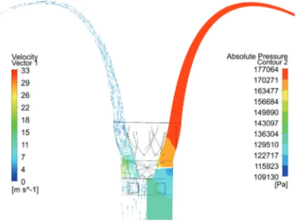
Fig. 5 Velocity vectors (left) and pressure contours (right) of the axial-flow pump model B at maximum efficiency point
Fig. 6 Pressure distribution across the pump models A and B at maximum efficiency point
Figure 4 shows the efficiency comparison of the two pump models. The pump models A and B have similar maximum efficiency of 84% at little different flow rates of 0.800 and 0.825m3/s, relatively. However, at the range of partial flow rate, the efficiency of the pump model B is relatively lower than that of the pump model A. Moreover, at the range of excessive flow rate, the efficiency of the pump model B shows higher value than that of the pump model A. These results indicate that the outlet shape has some influence to the performance and internal flow of the pump in the ranges of partial and excessive flow rate but almost same efficiency at the maximum efficiency point if the cross sectional area at the pump inlet remains same.
3.2. Pressure and velocity distributions
Figure 5 shows the pressure contours and velocity vectors of the axial-flow pump model B at the best
efficiency point. From the pressure contours, it is seen that the pressure increases gradually from the pump inlet to pump outlet, expecially sharp increase at the locations of impeller and diffuser guide vane.
Moreover, the velocity vectors show that the flow gains high velocity at the location of impeller.
For the more detailed quantitative examination of the pressure change in the pump flow passage, the static pressure distribution across the flow passage of the pump models A and B is shown in Fig. 6. It is clear that static pressure decreases a little in front of the impeller inlet because of the influence of swirl flow at the region, where position “0” in the Fig. 6 means impeller inlet. However, the pressure increases considerably after the impeller inlet and then, the pressure increases gradually from the diffuser guide vane to the pump outlet.
It can also be seen that there is almost no difference of the pressure distribution between the original (Type A) and the modified (Type B) pump models. This is because, although the outlet shape is changed, the cross sectional area of the pump inlet remains the same and hydraulic loss at the pump discharge shows no difference from the both pump models.
Moreover, the results show that the static pressure distribution lies over the saturation pressure line across the all flow passages from the inlet to the outlet of the pump models, which means that the possibility of cavitation occurrence is very low and cavitation performance is satisfactory.
3.3. Cavitation performance
In order to investigate the cavitation performance in detail, comparison of local static pressure on the impeller surface, where the possibility of cavitation occurrence is most high, with saturation pressure of the working fluid is conducted as shown in Fig. 7. The results show that the pressure on the blade surface is changing along the circumferential position of the pump and the pressure distribution of the impeller blades is almost same regardless of the blade location.
Moreover, the pressure distribution shows that pressure on the impeller blade surface is higher than the saturation pressure, so the occurrence of cavitation is very low.
Fig. 7 Static pressure distribution on the impeller blade surface of the pump model B at maximum efficiency point
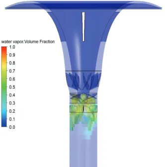
Fig. 8 Air volume fraction across axial-flow pump model B at maximum efficiency point
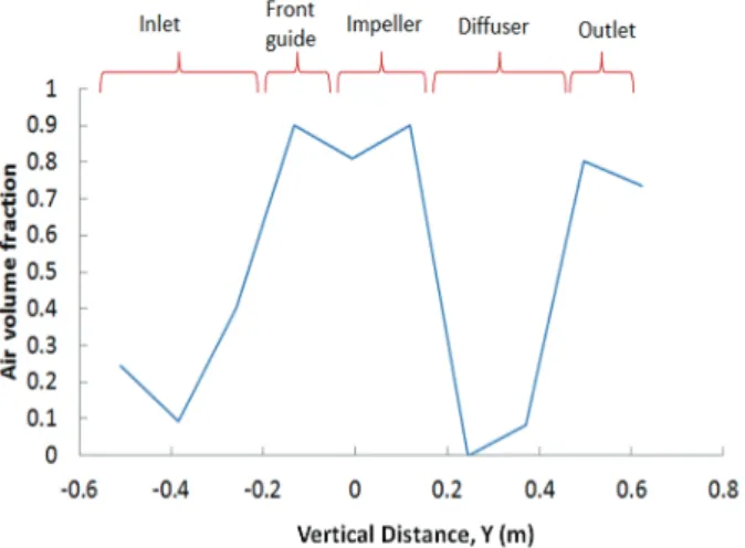
Fig. 9 Measuring locations of air volume fraction
The cavitation model in CFD analysis is based on the assumption that the water and vapor mixture in the cavitating flow can be modeled as a homogeneous fluid. Therefore, present study adopts the Rayleigh- Plesset Model(9) as a cavitation model, which illustrates cavitation by using the air volume fraction method.
Figure 8 shows the air volume fraction across axial-flow pump model B at the best efficiency point.
The value of volume fraction 1 means that air bubbles are completely formed and cavitation occurs and the value of 0 means there is only water. The values between 1 and 0 is a mixture. The results show no significant possibility of cavitation occurrence in the pump passage even though the values of the volume fraction in the regions between inlet guide vane and impeller is relatively higher than that of the other region.
Furthermore, for the purpose of investigating the possibility of cavitation occurrence in the pump passage in detail, measuring locations of the impeller surface, impeller shaft surface and whole flow passage are examined as shown in Fig. 9.
Figure 10 shows the air volume fraction on the impeller blade of pump model B at the best efficient point. The abscissa x/X represents local dimensionless chord length of the impeller blade, where x is length from leading edge to trailing edge and X is the chord length. The distribution of air volume fraction indicates that on the surface of the impeller blade, at the location of x/X=0.25, shows relatively higher value of air volume fraction but the value is below 0.35, which means very low possibility of cavitation occurrence.
Moreover, Fig. 11 shows the air volume fraction on the impeller shaft surface of pump model B at the best efficiency point. The value of air volume fraction in the region shows blow 0.6, which means low possibility of cavitation occurrence as well.
Figure 12 shows the distribution of the air volume fraction across flow passage of pump model B. The abscissa Y represents the vertical distance with origin at the impeller inlet. The result reveals relatively high value below 0.9 existing at the locations between the front guide vane and impeller. However, there is
still allowance from the margin of the cavitation occurrence.
Fig. 10 Air volume fraction on the impeller blade surface of pump model B at maximum efficiency point
Fig. 11 Air volume fraction on the impeller shaft surface of pump model B at maximum efficiency point
Fig. 12 Air volume fraction across flow passage of pump model B at maximum efficiency point
4. Conclusions
The study concludes that an efficient axial pump for floating type water treatment system is developed for oxygenating the deeper layer waters by mixing it with the surface air. The new outlet shape for aiding in simple floating structure is acceptable, contributing to a efficiency of 84% at the maximum efficiency point and a head of 4.8m.
The pump performance for model B does not change at the maximum efficiency point in contrast to model A, however, the efficiency of the pump decreases at the partial flow rate and increases at the excessive flow rate if the discharge passage is modified from model A to B for the floating type water treatment system.
The distribution of air volume fraction in the pump passage confirms that there may be low possibility of occurrence of cavitation in the pump system. Relatively high value of air volume fraction exists at the locations between the front guide vane and impeller but there is still allowance from the margin of the cavitation occurrence.
Acknowledgment
This work is financially supported by the Ministry of Trade, Industry & Energy (MOTIE), Republic of Korea through the fostering project of industry – university convergence.
References
(1) Cong, H. B., Huang, T. L., Chai, B. B., and Zhao, J. W., 2009, “A New Mixing-oxygenating Technology for Water Quality Improvement of Urban Water Source and its Implication in a Reservoir,” Renewable Energy, 34:
pp. 2054∼2060.
(2) Lawson, R. and Anderson, M. A., 2007, “Stratification and mixing in Lake Elsinore, California: An assessment of axial flow pumps for improving water quality in a shallow eutrophic lake,” Water Research, Vol. 41, pp.
4457∼4467.
(3) Yun, J. E., 2013, “Development of Submersible Axial Pump for Wastewater,” Trans. Korean Soc. Mech. Eng.
B, Vol. 37, No. 2, pp. 149∼154.
(4) Baek, S. H., Jung, W. H. and Kang, S. M., 2012, “Shape Optimization of Impeller Blades for Bidirectional Axial Flow Pump,” Trans. Korean Soc. Mech. Eng. B, Vol.
36, No. 12, pp. 1141∼1150.
(5) Park, H. C., Kim, S., Yoon, J. Y. and Choi, Y. S., 2012,
“A Numerical Study on the Performance Improvement of Guide Vanes in an Axial-flow Pump,” Journal of Fluid Machinery, Vol. 15, No. 6, pp. 58∼63.
(6) Kim, M. H., Kim, J. H. and Park J. S., 2001, “Prediction of Axial Pump Performance Using CFD Analysis,”
Journal of Computational Fluids Engineering, Vol. 6, No.
1, pp. 14∼20.
(7) Choi, Y. S., Lee, K. Y., Lee, C. H. and Lee J. H, 2003,
“Development of Leakage-free Automatic Discharge Connector in a Submersible Pump,” Journal of Fluid Machinery, Vol. 6, No. 2, pp. 23∼28.
(8) Zhang, D. S., Shi, W. D., Chen, B. and Guan, X. F., 2010, “Unsteady Flow Analysis and Experimental Investigation of Axial-flow Pump,” Journal of Hydrodynamics, Vol. 22, No. 1, pp. 35∼43.
(9) McAliley, I. E. and D’Adamo, P., 2010, “Reservoir Mixing to Enhance Raw Water Quality and Treatability,”
NC AWWA-WEA Annual Conference Technical Papers.
(10) ANSYS Inc, 2013, “ANSYS CFX Documentation,” Ver.
14, http://www.ansys.com
(11) Lakshminarayana, B., 1991, “An Assessement of Computational Fluid Dynamic Techniques in the Analysis and Design of Turbomachinery : The 1990 Freeman Scholar Lecture,” ASME Journal of Fluids Engineering, Vol. 113, pp. 315∼352.