MATHEMATICAL MODELING OF CHEMICAL PROCESS

(1)

CHE302 Process Dynamics and Control Korea University ^4-1

CHE302 LECTURE IV

MATHEMATICAL MODELING OF CHEMICAL PROCESS

Professor Dae Ryook Yang

Fall 2001

Dept. of Chemical and Biological Engineering Korea University

THE RATIONALE FOR MATHEMATICAL MODELING

• Where to use

– To improve understanding of the process – To train plant operating personnel

– To design the control strategy for a new process – To select the controller setting

– To design the control law

– To optimize process operating conditions

• A Classification of Models

– Theoretical models (based on physicochemical law) – Empirical models (based on process data analysis) – Semi -empirical models (combined approach)

DYNAMIC VERSUS STEADY-STATE MODEL

• Dynamic model

– Describes time behavior of a process

• Changes in input, disturbance, parameters, initial condition, etc.

– Described by a set of differential equations

: ordinary (ODE), partial (PDE), differential-algebraic(DAE)

• Steady-state model

– Steady state: No further changes in all variables – No dependency in time: No transient behavior

– Can be obtained by setting the time derivative term zero

Dynamic Model (ODE, PDE) Initial Condition, x(0)

Input, u(t) Output, y(t)

Parameter, p(t)

MODELING PRINCIPLES

• Conservation law

– Within a defined system boundary (control volume)

• Mass balance (overall, components)

• Energy balance

• Momentum or force balance

• Algebraic equations: relationships between variables and parameters

rate of rate of rate of accumulation input output

rate of rate of generation disappreance

     

= −

     

     

   

+  − 

   

(2)

MODELING APPROACHES

• Theoretical Model – Follow conservation laws – Based on physicochemical

laws

– Variables and parameters have physical meaning – Difficult to develop – Can become quite complex – Extrapolation is valid unless

the physicochemical laws are invalid

– Used for optimization and rigorous prediction of the process behavior

• Empirical model

– Based on the operation data – Parameters may not have

physical meaning – Easy to develop – Usually quite simple – Requires well designed

experimental data

– The behavior is correct only around the experimental condition

– Extrapolation is usually invalid

– Used for control design and simplified prediction model

DEGREE OF FREEDOM (DOF) ANALYSIS

• DOF

– Number of variables that can be specified independently – N_F = N_V- N_E

• N_F: Degree of freedom (no. of independent variables)

• N_V: Number of variables

• N_E: Number of equations (no. of dependent variables)

• Assume no equation can be obtained by a combination of other equations

• Solution depending on DOF

– If N_F= 0, the system is exactly determined . Unique solution exists.

– If N_F> 0, the system is underdetermined. Infinitely many solutions exist.

– If N_F< 0, the system is overdetermined. No solutions exist.

LINEAR VERSUS NONLINEAR MODELS

• Superposition principle

• Linear dynamic model:superposition principle holds

– Easy to solve and analytical solution exists.

– Usually, locally valid around the operating condition

• Nonlinear: “Not linear ”

– Usually, hard to solve and analytical solution does not exist.

1 2 1 2

, , and for a linear operator,

Then ( ( ) ( )) ( ( )) ( ( )) L

L x t x t L x t L x t

α β

α β α β

∀ ∈ℜ

+ = +

1 1 2 2

1 2 1 2

1 1 2 2

1 2 1 2

, , ( ) ( ) and ( ) ( )

( ) ( ) ( ) ( )

, , (0) ( ) and (0) ( )

(0) (0) ( ) ( )

u t y t u t y t

u t u t y t y t

x y t x y t

x x y t y t

α β

α β α β

α β

α β α β

∀ ∈ℜ → →

+ → +

∀ ∈ℜ → →

+ → +

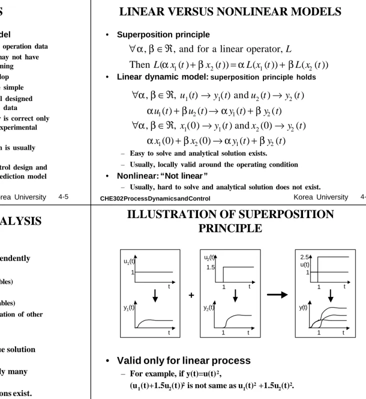
ILLUSTRATION OF SUPERPOSITION PRINCIPLE

• Valid only for linear process

– For example, if y(t)=u(t)²,

(u₁(t)+1.5u₂(t))²is not same as u₁(t)² +1.5u₂(t)².

u₁(t)

t 1

y₁(t)

t

u₂(t)

t 1.5

1

y₂(t)

t 1

y(t)

t 1 u(t)

t 2.5

1 1

+

(3)

TYPICAL LINEAR DYNAMIC MODEL

• Linear ODE

• Nonlinear ODE

( ) ( ) ( ) ( and K are contant, 1st order) dy t y t Ku t

τ dt = − + τ

1

1 1 0

1

1 1 0

( ) ( )

( )

( ) ( )

() (nth order)

n n

n n n

m m

m m m m

d y t d y t

a a y t

dt dt

d u t d u t

b b b u t

dt dt

−

− −

−

− −

+ + +

= + + +

K

( ) 2

( ) ( )

dy t y t Ku t τ dt = − +

( ) ( ) ( )

dy t y t K u t τ dt = − +

( ) ( ) ( ) s i n ( ) ( ) dy t y t y t y Ku t

τ dt = − +

( ) ( )

y t ( )

dy t Ku t

dt

e

τ = − ⁻ +

MODELS OF REPRESENTATIVE PROCESSES

• Liquid storage systems

– System boundary: storage tank – Mass in: q_i(vol. flow, indep. var) – Mass out: q (vol, flow, dep. var) – No generation or disappearance

(no reaction or leakage) – No energy balance

– DOF=2 (h, q_i) - 1=1

– If , the ODE is linear.

(R_V is the resistance to flow)

– If , the ODE is nonlinear.

(C_Vis the valve constant)

i i

( )

A dh q q q f h dt

= − = −

Accumulation rate in tank

Mass in rateMass out rate Outlet flow is a function of head ( ) / V

f h =h R

( ) V / c

f h =C ρgh g

h V q_i

q Area = A

Control volume

• Continuous Stirred Tank Reactor (CSTR) – Liquid level is constant(No acc. in tank)

– Constant density, perfect mixing – Reaction: A à B (r = k₀exp (-E/RT)c_A) – System boundary: CSTR tank

– Component mass balance

– Energy balance

– DOF analysis

• No. of variables: 6 ( q, c_A, c_Ai, T_i, T, T_c)

• No. of equation:2 (two dependent vars.: c_A, T)

• DOF=6 – 2 = 4

• Independent variables: 4 ( q, c_Ai, T_i, T_c)

• Parameters: kinetic parameters, V, U, A, other physical properties

• Disturbances: any of q, c_Ai, T_i, T_c, which are not manipulatable h V, T c_Ai, q_i, T_i

Cooling medium,Tc

cA, q, T

( )

A

Ai A A

V dc q c c Vkc

dt

= − −

( ) ( ) ( )

p p i A c

V C dT q C T T H Vkc U A T T

ρ dt

=

ρ

− + −∆ + −

STANDARD FORM OF MODELS

• State-space model

– x: states, [c_AT]^T – u: inputs, [q T_c]^T

– d: disturbances, [c_AiT_i]^T

– y: outputs – can be a function of above, y=g(x,d,u), [c_AT]^T – If higher order derivatives exist, convert them to 1^storder.

1 1 1

/ ( , , )

where [ , ,

_n

] ,

^T

[ , ,

_m

] ,

^T

[ , ,

_l

]

^T

d dt

x x u u d d

= =

= = =

x x f x u d

x u d

&

L L L

1

2

( ) ( , , , )

( ) ( ) ( ) ( , , , , )

A

Ai A A A Ai

i A c A c i

p p

dc q

c c kc f c T q c dt V

dT q q UA

T T H kc T T f c T q T T

dt V ρC ρC

= − − =

= − + −∆ + − =

From the previous example

(4)

CONVERT TO 1

^ST

-ORDER ODE

• Higher order ODE

• Define new states

• A set of 1

^st

-order ODE’s

1

1 1 0 0

( ) ( )

n n

n n n

d x t d x t

a a x t b u t

dt dt

−

− −

+ + +

K

=

( 1) 1

, , , ,

2 3 _n ⁿ

x = x x = x x & = & x &L x = x

⁻

1 2

2 3

1 2 1 0 1 0

n n n n n

x x

x a

₋

x a

₋

x

₋

a x b u

=

= − − − − +

&

M

& L

SOLUTION OF MODELS

• ODE (state-space model)

– Linear case: find the analytical solution via Laplace transform, or other methods.

– Nonlinear case: analytical solution usually does not exist.

• Use a numerical integration, such as RK method, by defining initial condition, time behavior of input/disturbance

• Linearize around the operating condition and find the analytical solution

• PDE

– Convert to ODE by discretization of spatial variables using finite difference approximation and etc.

1 ( )

L L

w L

HL

T T

v T T

t z τ

∂ = − ∂ + −

∂ ∂

( ) ( 1)

L L L

T T j T j

z z

∂ ≈ − −

∂ ∆

( ) 1 1

( 1) ( )

( 1, )

L

L L w

HL HL

dT j v v

T j T j T

dt z z

j N

τ τ

 

= −∆ − −∆ +  +

= L

LINEARIZATION

• Equilibrium (Steady state)

– Set the derivatives as zero:

– Overbar denotes the steady-state value and is the equilibrium point. (could be multiple)

– Solve them analytically or numerically using Newton method

• Linearization around equilibrium point

– Taylor series expansion to 1^storder

– Ignore higher order terms – Define deviation variables:

( , , )

=

0 f x u d

( , , )x u d

( , ) ( , )

( , ) ( , ) ∂ ( ) ∂ ( )

= + − + − +

∂ _{x u} ∂ _{x u}

f f

f x u f x u x x u u

x u L

0

( , ) ( , )

∂ ∂

′= ′+ ′= ′+ ′

∂ _{x u} ∂ _{x u}

f f

x x u Ax Bu

x u

&

′= − , ′= −

x x x u u u

1 1

1

n

n n

n

f f

x x

f f

x x

∂ ∂

 

∂ ∂ 

 

∂ =  

∂ ∂ ∂ 

∂ ∂ 

 

f x

L

M O M

L Jacobian