https://doi.org/10.5228/KSTP.2019.28.2.89
Process Metamorphosis and On-Line FEM for Mathematical Modeling of Metal Rolling-
Part II: Application
A. Zamanian1, S.Y. Nam1, T. J. Shin1, S. M. Hwang#
(Received January 14, 2019 / Revised March 13, 2019 / Accepted March 15, 2019)
Abstract
In this paper, we examine the application of a new concept – on-line FE model in various metal rolling processes. This technology allows for completion of process simulation within a tiny fraction of a second without losing the high level of prediction accuracy inherent to FEM. The procedure is systematically demonstrated through the design of actual on-line models for the prediction of the width spread in horizontal rolling of the slab using a dog bone profile and horizontal rolling of the strip with a strip profile. The validity and the prediction accuracy of the on-line FE models were analyzed and discussed.
Key Words: Process Metamorphosis, Hypothetical Process, Width Spread, Finite Element Method, On-line Model
1. Introduction
Deformation occurring in metal rolling is a three dimensional, non-steady process. As a result, it is not uncommon for process simulation of flat rolling, when carried out on the basis of FEM [1-2], to take hours and days before it would finally come to an end. Therefore, it is impossible to implement FEM for on-line mill setup and control on the production line.
In part I of this paper, the new concept – on-line FE model is described in detail, and the procedure is demonstrated step by step through designing actual on-line models for the prediction of the dog-bone profile in edge rolling.
In this paper, the procedure is described step by step through designing actual on-line models for the prediction
of the width spread in horizontal rolling of the slab with a dog bone profile as well as in horizontal rolling of the strip with a strip profile. The validity and the prediction accuracy of the on-line FE models are examined and discussed.
2. Design of an on-line FE model for the prediction of width spread in horizontal rolling of the slab with a dog bone profile
The number of elements and the number of time steps that have to be employed for FE process simulation of horizontal rolling of the slab with a dog bone profile are 30,000 and 2,500 respectively, as illustrated in Fig 1.
Therefore, it is highly desired to have an on-line FE model for the prediction of width spread.
1. Department of Mechanical Engineering, POSTECH
# Corresponding Author: Department of Mechanical Engineering, POSTECH, E-mail: [email protected],
ORCID ID: 0000-0001-9347-4472
Fig. 1 Original FE mesh selected for process simulation of horizontal rolling of the slab with a dog-bone profile (a) before rolling, b) after rolling
Step 1.
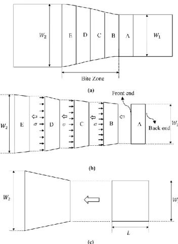
The target parameter to be considered in process metamorphosis is the width spread that may be predicted from FE simulation of horizontal rolling. As illustrated in Fig. 2, steady-state deformation occurring in the bite zone may be replaced by progressive compression of a narrow piece. At each stage of the progressive compression of a piece, fromAtoE, the lateral displacement should not be allowed to occur at its back end. Process metamorphosis into progressive compression of a narrow piece, however, is not viable, since the compressive stress to be applied to the front end of the piece at each stage is not known. This
problem may be resolved by metamorphosing the process of progressive compression of a narrow piece into flat die compression of a block, as follows.
Fig. 2 Process metamorphosis. (a) the original process - horizontal rolling, (b) The process obtained by metamorphosis of horizontal rolling- progressive compression of a narrow piece, (c) the process obtained by metamorphosis of progressive compression of a narrow piece - flat die compression of a block
The initial dimensions of the block to be compressed between the upper die and the lower die should precisely reflect the entry thicknessH1, dog-bone profile, and the entry width W1 of the slab before rolling. Regarding the length of the block, it may be determined from step 3. The block is to be compressed until the delivery thicknessH2 is achieved.
The back end of the block represents the roll entry. It is in this regard that a special boundary condition is applied to
the back end of the block so as to prohibit the lateral displacement while being compressed between the flat dies, as shown in Fig. 3
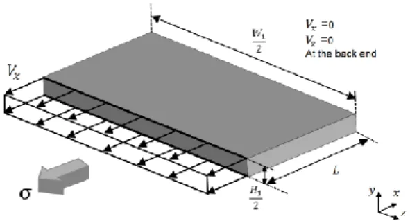
Fig. 3 A hypothetical process. The slab with a dog-bone profile is to be compressed between two flat dies, with special boundary conditions applied to the back end and to the line of symmetry (line A) at the front end
The front end of the block represents the roll exit. A special boundary condition is applied to the line of symmetry at the front end of the block, which is depected as line A in Fig. 3 Line A is to move along the rolling direction uniformly with the speed Vx. The speed may be determined by the condition that the resultant force to be applied to the line is zero. This boundary condition is designed to induce the front end of the block to replicate the steady-state cross-section of the material exiting the roll gap in horizontal rolling, at the completion of flat die compression.
Regarding the friction acting at the die–block interface, the same friction as used in FE simulation of rolling may be applied. It is assumed that the coefficient of Coulomb friction is0.3.
The delivery width W2is regarded as the width of the bottom line of the front end of the compressed block, which is on the line of symmetry.
Step 2.
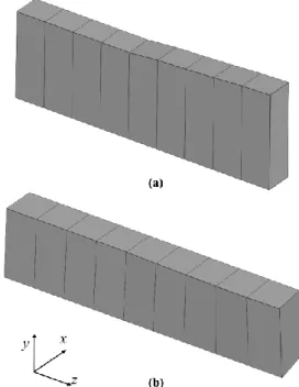
The mesh selected for FE simulation of the compression of a block between the two flat die compressions is shown in Fig. 4 Due to the symmetry, only a quarter of the block need to be considered. Nine elements are deployed across
the width direction, and one element is deployed across the thickness direction. The number of elements is nine, which is in stark contrast to the the number of elements used in FE simulation of horiozntal rolling. The number of time steps selected is 30, which is also a tiny fraction of the number of time steps required for FE simulation of horizontal rolling.
Fig. 4 On-line FE mesh selected for simulation of the hypothetical process (a) before compression, (b) after compression
Step 3.
It turns out that the plain carbon steel is again too soft to withstand the extremity of the boundary conditions imposed on the line A, leading to failure in obtaining the solution convergence. The material for the hypothetical process, which is selected on the basis of the predictions from a series of FE simulation, has the constant yield stress of Y= 5 GPa. Note that such an unrealistic material is perfectly acceptable, as implied by the word hypothetical.
Regarding the initial length of the block, L= 45 mm is selected. Note that the yield stress as well as the initial length of the block may vary with the carbon content and temperature.
Application.
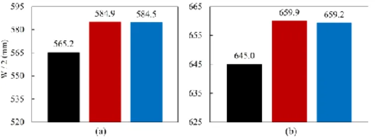
The process conditions considered to examine the validity of the on-line model are described in Table 1. The computation time required for simulation with the on-line FE model is less than 0.1 second. Predictions from the on- line FE model are in excellent agreement with predictions from FE simulation of edge rolling, as illustrated in Fig. 5 It is interesting to note that a single set of constants representing Y and L can cover a wide range of rolling conditions as listed in Table 1
Fig. 5W2/ 2
, from original FE simulation ( ), from on-line FE model ( ),
W1/ 2( ). Process conditions are, (a) case A2-L-H, (b) case B-H in Table 1
Table 1 Process conditions selected for horizontal rolling of the slab with a dog bone profile
Case FEM On-Line FEM
Edge Rolling
Horizontal Rolling
H 1
(mm) H 2
(mm) R (mm)
W 1
(mm) L (mm)
Y (GPa)
A1-S A1-S-H 192 150 650 1623.0 45.0 5.0
A2-S A2-S-H 214.6 165 650 1210.0 45.0 5.0
C C-H 143 112 657.5 1072.0 45.0 5.0
A3-S A3-S-H 280 230 650 928.0 45.0 5.0
B B-H 160 128 575 1290.0 45.0 5.0
A1-L A1-L-H 192 150 650 1523.0 45.0 5.0
A3-L A3-L-H 280 230 650 881.0 45.0 5.0
A2-L A2-L-H 214.6 165 650 1130.4 45.0 5.0
3. Design of an on-line FE model for the prediction of width spread in horizontal rolling of the strip with a strip profile.
The number of elements and the number of time steps that have to be employed for FE process simulation of horizontal rolling of the strip with a strip profile profile are 50,000 and 5,000 respectively, as illustrated in Fig. 6 Therefore, it is highly desired to have an on-line FE model for the prediction of width spread.
(a)
(b)
Fig. 6 Original FE mesh selected for process simulation of horizontal rolling of the strip with a strip profile. (a) Before rolling, b) after rolling
Step 1.
The target parameter to be considered in process metamorphosis is the width spread that may be predicted from FE simulation of horizontal rolling conducted in a hot strip mill. As in the case of horizontal rolling of the slab with a dog-bone profile, the process may also be
metamorphosed into flat die compression of a block, with some modifications.
The initial dimensions of the block to be compressed between a couples of flat dies must precisely reflect, the entry strip profileC z1( )H1(0)H z1( ), the entry width of the strip W1 and the entry thicknessH1(0)before rolling.
Regarding the length of the block, it may be determined from step 3. The block is to be compressed until the delivery thickness H2(0) is achieved.
A contoured die should be used in stead of a flat die so as to imprint the delivery strip profile on the block after compression. C z2( )H2(0)H z2( )
The back end of the block is subject to a special boundary condition that prohibits the lateral displacement while being compressed between the flat dies, as shown in Fig. 7
Fig. 7 A hypothetical process. The strip with a strip profile is to be compressed between two flat dies, with special boundary conditions applied to the back end as well as to the front end
The entire front end of the block is forced to move along the rolling direction uniformly with an identical speedVx, as shown in Fig. 7. The speed may be determined by prescribing the resultant force to be applied to the front end.
The boundary conditions are designed to induce the front end of the block to replicate the steady-state cross-section of the rolled strip, at the completion of the compression process.
Regarding the friction acting at the die–block interface, the same friction as used in FE simulation of rolling may be applied. It is assumed that the coefficient of Coulomb friction is0.3.
The delivery width W2is regarded as the average width of the the front end of the compressed block.
Step 2.
The mesh selected for FE simulation of the compression of a block between the two flat die compressions is shown in Fig. 8 Due to the symmetry, only a quarter of the block need to be considered. Nine elements are deployed across the width direction, and one element is deployed across the thickness direction. The number of elements is nine, which is in stark contrast to the the number of elements used in FE simulation of horizontal rolling. The number of time steps selected is 30, which is also a tiny fraction of the number of time steps required for FE simulation of horizontal rolling.
(a)
(b)
Fig. 8 On-line FE mesh selected for simulation of the hypothetical process (a) before compression, (b) after compression
Step 3.
Regarding the material, the flow stress characteristics of the block should be the same as those of the strip to be rolled.
Regarding the die speed, it may be selected such that the compression process is complete at the moment a material particle arrives at the roll exit. In this way, the effect of
2 1 1
1 1
( , , )
W W W
W f r l H
2 1 1
1 1
( , , )
W W W
W g r L H
strain rate on the flow stress characteristics of the material may be reflected.
Regarding the initial length of the block, it may be determined as follows.
We may consider a dimensionless form of an equation representing the relation between the process variables defining the geometry of horizontal rolling.
(1)
Whererdenotes the reduction ratio, and l denotes the bite zone length.
In flat die compression, Equation 1 may be replaced by
(2)
WhereLdenotes the initial length of the block.
Considering that whenW1,l and H1 are given, 2
1
W W is governed only byr, we may assume that
(3)
Similarly, we may assume that for flat die compression
(4)
From the condition , we may obtain
(5)
Various forms of have been proposed by Siebel [4], Hill [5], Wusatowski [6], Sparling [7], Helmi [8], and Beese [9], in the following form.
(6)
Comparing with, it may be assumed that
(7)
β proposed by Helmi [8] may be adopted to derive, which is
(8)
Application 1. (Material: Y = 0.2 GPa)
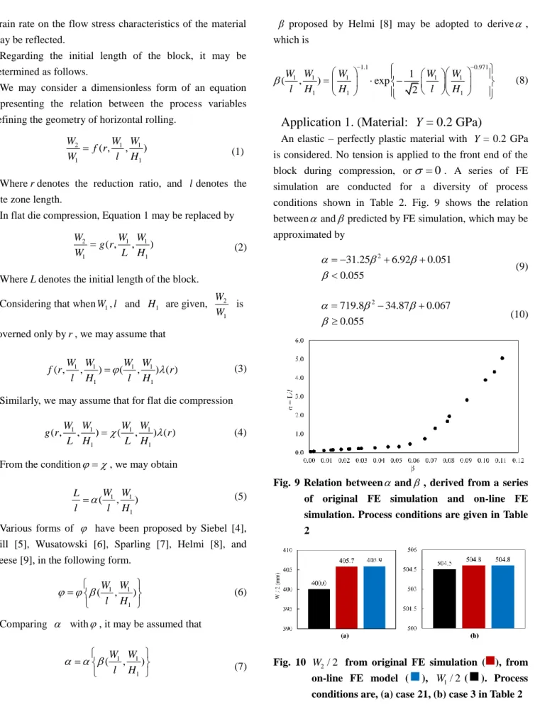
An elastic – perfectly plastic material with Y= 0.2 GPa is considered. No tension is applied to the front end of the block during compression, or 0. A series of FE simulation are conducted for a diversity of process conditions shown in Table 2. Fig. 9 shows the relation betweenandpredicted by FE simulation, which may be approximated by
(9)
(10)
Fig. 9 Relation between
and
, derived from a series of original FE simulation and on-line FE simulation. Process conditions are given in Table 2
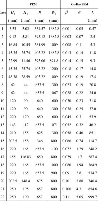
Fig. 10
W2/ 2from original FE simulation ( ), from on-line FE model ( ),
W1/ 2( ). Process conditions are, (a) case 21, (b) case 3 in Table 2
1 1 1 1
1 1
( ,W W, ) (W W, ) ( )
f r r
l H l H
1 1 1 1
1 1
( ,W W, ) (W W, ) ( )
g r r
L H L H
1 1
1
(W ,W ) L
l l H
1 1
1
(W W, ) l H
1.1 0.971
1 1 1 1 1
1 1 1
( , ) exp 1
2
W W W W W
l H H l H
1 1
1
(W W, ) l H
31.25 2 6.92 0.051 0.055
719.8 2 34.87 0.067 0.055
Table 2 Process conditions selected for horizontal rolling of a strip, Y = 0.2 GPa
Case
FEM On-line FEM
H1
(mm) H2 (mm)
R (mm)
W1
(mm)
L
(mm) 1 3.33 3.02 334.57 1682.8 0.001 0.05 0.57 2 9.12 5.81 393.12 1682.8 0.003 0.07 2.5 3 16.84 10.45 381.99 1009 0.008 0.11 5.3 4 45.35 25.74 403.22 1682.8 0.013 0.14 11.8 5 22.99 11.46 393.06 894.8 0.014 0.15 9.3 6 45.35 25.74 403.22 1200 0.018 0.17 14.8 7 48.38 28.59 403.22 1009 0.023 0.19 17.4 8 62 44 657.5 1300 0.023 0.19 20.8 9 62 44 657.5 1067 0.028 0.22 24.0 10 120 90 640 1600 0.030 0.23 31.8 11 120 90 640 1300 0.038 0.25 37.0 12 220 170 650 1600 0.045 0.31 53.9 13 143 112 657.5 1071 0.052 0.32 46.2 14 210 155 625 1300 0.058 0.46 85.1 15 202.5 158 346 800 0.066 0.74 114.7 16 220 165 657.5 1100 0.072 1.29 248.2 17 155 116.83 650 800 0.079 1.7 287.4 18 220 165 657.5 1000 0.080 1.94 364.9 19 220 165 657.5 900 0.091 2.81 534.7 20 202.5 148.4 675 800 0.101 3.88 746.4 21 250 195 657 800 0.106 4.31 854.6 22 250 190 657 800 0.111 5.05 999.7
The predictions from the on-line FE model are in excellent agreement with the predictions from the original FE simulation for various process conditions covering both the roughimg mill and the finishing mill, as illustrated in Fig. 10 Each computation takes less than 0.1 second.
Application 2. (Material = plain carbon steel)
A plain carbon steel is considered, the flow stress of
which is given by Misaka [3]. The initial length of the block is calculated from Equations 8, 9, and 10. A series of FE simulation are conducted for a diversity of process conditions shown in Table 3 It is found that, apart from replacing the material, a proper amount of tension has to be applied to the front end of the block in order to achieve the desired prediction accuracy. The relation between the tension andderived on the basis of the predictions from a series of FE simulation is given by
(11)
(12)
Where is in GPa, and when0.018, 0
Fig. 11
W2/ 2, from original FE simulation ( ), from on-line FE model ( ),
W1/ 2( ). Process conditions are case 13 in Table 3, (a) C =0.02%, T = 1200°C (b) C = 1% T = 1200°C (c) C = 0.02% T = 800°C
Fig. 12
W2/ 2, from original FE simulation ( ), from on-line FE model ( ),
W1/ 2( ). Process conditions are case 4 in Table 3, delivery strip crown is, (a) +480 µm , (b) -480 µ m, entry strip crown is 0 µ m for both (a) and (b)
( ) 30.25 2 4.26 0.066
0.018 0.055
( ) 10.49 2 0.87 0.011 0.055
As illustrated in Fig. 11, the on-line FE model as applied to the prediction of the width spread in a roughing mill manifests its sublime prediction accuracy, to the level even the effect of the carbon content and temperature is reflected.
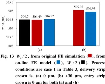
The effect of the strip crown can also be precisely reflected when applied to the prediction of the width spread in a finishing mill, as illustrated in Fig. 12 and Fig. 13
Table 3 Process conditions selected for horizontal rolling of a strip, plain carbon steel.
Case
FEM On-line FEM
H1 (mm)
H2 (mm)
R
(mm)
W1 (mm)
C
(%)
T
(°C)
L
(mm)
(GPa) 1 3.6 2.7 334.6 1009 0.034 910 0.002 0.062 1.1 0.0 2 9.1 5.8 315.1 1009 0.034 1200 0.004 0.081 2.6 0.0 3 21.1 14.2 381.9 1500 0.5 1000 0.007 0.095 4.9 0.0 4 45.3 25.7 403.2 1200 0.034 1200 0.018 0.169 14.8 0.001 5 62 44 657.5 1067 0.034 800, 1200 0.028 0.216 24.0 0.030 6 120 90 640 1600 0.02, 1 800, 1200 0.030 0.226 31.8 0.035 7 55.9 33.6 403.2 850 0.2 900 0.032 0.239 22.7 0.040 8 120 90 640 1300 0.034 800, 1200 0.038 0.255 37.0 0.053 9 220 170 650 1600 0.034, 1 800, 1200 0.045 0.316 53.9 0.065 10 143 112 657.5 1071 0.02, 1 800, 1200 0.052 0.319 46.2 0.074 11 210 155 625 1300 0.02, 1 800, 1200 0.058 0.458 85.1 0.096 12 220 165 657.5 1100 0.034 800, 1200 0.072 1.294 248.2 0.127 13 220 165 657.5 1000 0.02, 1 800, 1200 0.080 1.940 364.9 0.147 14 220 165 657.5 900 0.034 800, 1200 0.091 2.813 534.7 0.176 15 202.5 148.4 675 800 0.02, 1 800, 1200 0.101 3.883 746.4 0.205 16 250 190 657 800 0.034 800, 1200 0.111 5.047 999.7 0.236
4. Concluding remarks
It is demonstrated that an on-line FE model that would replace an original FE model can be derived from process metamorphosis, in a step by step manner. An original process may be metamorphosed into various hypothetical processes.
Fig. 13
W2/ 2, from original FE simulation ( ), from on-line FE model ( ),
W1/ 2( ). Process conditions are case 1 in Table 3, delivery strip crown is, (a) 0 µm, (b) +30 µ m, entry strip crown is 0 µm for both (a) and (b)
To be capable of finding the best one among them in the light of the prediction accuracy and computational efficiency may depend on the designer’s experience and intuition. It is expected that the technology demonstrated in this paper may find application in diverse fields of science and engineering and serve as a powerful tool leading to next generation on-line models.
Acknowledgements
This work was supported by the National Research Foundation of Korea (NRF) grant funded by the Korea government (MSIP) (No.2012R1A5A1048294).
REFERENCES
[1] J. S. Lee, T. J. Shin, S. J. Yoon, S. M. Hwang, 2016, Prediction of Steady-state Strip Profile in Flat Rolling, Steel Res. Int., Vol.87, No. 7, pp. 930~940.
[2] H. J. Park, S. M. Hwang, 2017, 3-D Coupled Analysis of Deformation of the Strip and Rolls in Flat Rolling by FEM, Steel Res. Int., Vol.88, No. 12, pp. 1700227 (1~13).
[3] Y. Misaka, T. Yoshimoto, 1967, Formulation of mean resistance of deformation of plain carbon steel at elevated temprature, J. Jpn Soc. Technol. Plast., Vol.8, No. 79, pp. 414~422.
[4] E. Siebel, 1932, Forming in plastic state: theoretical foundations of technical forming processes, Stahleisen, Düsseldorf, p. 91.
[5] R. Hill, 1950, A comparative study of some variational principles in the theory of plasticity, J.
Appl. Mech., Vol. 17, p. 64.
[6] Z. Wusatowski, 1955, Hot Rolling; A Study of Draft, Spread and Elongation, Iron and Steel, Vol. 28, pp.
89~94.
[7] L. G. M. Sparling, 1961, Formula for ‘Spread’ in Hot Flat Rolling, Proc. Instn. Mech. Engrs, Vol. 175 , pp.
604.
[8] A. Helmi, J. M. Alexander, 1968, Geometric factors affecting spread in hot flat rolling of steel, J. the Iron and Steel Inst., No. 206, pp. 1110~1117.
[9] J. G. Beese, 1972, Nomograms for predicting the spread of hot rolled slabs, AISE Yearly Proceedings, pp. 251~252.