The Impacts of Biofuel Production on Water Quality and a Mitigation Methodology to Reduce the Impacts

* Research Scientist, Spatial Science Laboratory, Texas A&M University, College Station, TX, USA, [email protected]

The Impacts of Biofuel Production on Water Quality and a Mitigation Methodology to Reduce the Impacts

Taesoo Lee*

바이오 연료 생산이 수질에 미치는 영향과 수질오염의 최소화 방안

이태수*

Abstract：Biofuel crops and their economical benefits have been recently researched as one of the alternative energy sources. Very few studies, however, have brought an issue about the impacts of the new cropping on environment, especially water quality. Because biofuel cropping requires more crop production with more fertilizers for cost- effectiveness, water quality near the new crops as well as downstream is expected to be degraded.

In this study, the impacts of biofuel crop production on water quality was estimated by scenarios between pre- biofuel cropping and post-biofuel cropping using the previously calibrated SWAT (Soil and Water Assessment Tool) model in a watershed in Texas, USA. Then, 30 meter filter strips were implemented on each biofuel ropland as a mitigation method. The economical and agricultural aspect and requirements of biofuel cropping was also previously investigated. The on-site impacts estimation showed that biofuel cropping increased about 250% to 1,150% of Total Nitrogen and about 100% to 1,100% of Total Phosphorous annually. The off-site estimation at the reservoir (entire watershed outlet) showed the annual increase of 40 to 50% for both Total Nitrogen and Total Phosphorous. The on-site effectiveness of filter strips was from 58.0% to 67.9% reduction for Total Nitrogen and 57.7% to 68.2% reduction for

Total Phosphorous. The filter strips reduced 28.5% of Total Nitrogen and 29.4% of Total Phosphorous at the watershed outlet.

Key Words : Biofuel, SWAT, Total Nitrogen, Total Phosphorous, Water quality

요약：대체에너지로써의 바이오 연료 작물과 그 경제성에 대한 연구가 최근 활발히 진행되고 있다. 하지만 이러한 새로운 작물의 생 산에 따른 수질변화에 대한 연구는 거의 없는 실정이다. 바이오 연료 작물은 그 경제적 효율성 때문에 많은 양의 비료를 필요로 하므 로 농경지 부근과 하류지역의 수질 오염이 예측된다. 이 논문에서는 바이오 연료 작물이 수질에 미치는 영향을 검정된 SWAT (Soil and Water Assessment Tool)모델을 이용하여 작물의 전과 후의 시나리오로 예측하였다. 그리고 수질 악화를 줄이는 방안으로 30미 터 넓이의 필터 스트립을 모델에서 시뮬레이션 하였다. 바이오 연료 작물 생산에 필요한 농경 일정은 이 전의 연구를 참고하였다. 모 델 예측 결과, 농경지 주변에서는 연간 250-1,150%의 총질소가, 그리고 100-1,100%의 총인이 각각 증가하였다. 유역의 유출구 (호 수)에서는 연간 40-50%의 총질소와 총인이 증가하였다. 필터 스트립을 설치한 후 농경지 주변에서는 연간 58.0-67.9%의 총질소와 57.7-68.2%의 총인이 각각 감소하였으며 유출구에서는 연간 28.5%의 총질소와 29.4%의 총인이 각각 감소하였다.

주요어 : 비이오 연료, SWAT, 총질소, 총인, 수질

1. Introduction

Bioenergy and its economical benefits have been researched as one of the alternative energy sources that solve or mitigate the concerns of rapidly increased fossil fuel consumption, rise of its price, and future depletion. After the energy crossroads of the State of Texas in 90s where consumption of energy became larger than production, bioenergy has been a greater interest.

The state of Texas in the US, for example, is the largest state in consumption of energy, natural gas, petroleum, and other energy sources among other states, it is nearly the last one in usage of renewable energy (Virtus-Energy- Research-Associates, 1995). Thus, prior to the commencement with biofuel production operation, statewide evaluation for biofuel crop potential is important and necessary to maximize effectiveness as well as to minimize environ mental impacts.

Texas has the largest cropland area as well as CRP (Conservation Reserve Program) land in the US and the CRP land (about 1.6 million hectares) will be released from the program in the next 5 to 10 years. These lands can be primary candidates for biofuel crop production. Nutrient condition in soil and water availability for crop production is critical because biomass yield depends heavily on those factors. For example, a fertile field can yield 30 times larger than an infertile one; and wide range of weather condition in Texas, which varies from arid to forested land, limits crop production and requires water supply. Also, a tremendous amount of fertilizer application will be expected and necessary to maximize the yields for cost effectiveness and profits of producers.

Very few studies, however, have been conducted to investigate the impacts by changes of landuse and agricultural operation on

environments. The conversion of crop type from rangeland to switchgrass (one of the biofuel crops) and the increased amount of fertilizer application can aggravate the environment dramatically, especially water quality. In this respect, a comprehensive study through a modeling approach that takes into account spatial variation such as detailed soil information, land cover changes, and climate variability is important and critical to assess environmental impacts by the production of those crops.

Therefore, the objectives of this study are 1) to set up a biofuel crop production (switchgrass) by conversion from original landuse (rangeland) to switchgrass in a previously calibrated model in the Eagle Mountain watershed, Texas, USA, 2) to assess the impacts of the newly adopted crop on water quality by pre- and post scenarios, and 3) to estimate the effectiveness of filter strips to reduce pollutants (Total Nitrogen and Total Phosphorous) that was increased by biofuel crop production in the watershed.

This study introduced biofuel crops, their necessary agricultural operations, and the role of filter strips through the review of the previous studies, then, showed the previous modeling works including calibration and validation of SWAT model, and finally analyzed the negative impacts of biofuel crops as well as the positive impacts of filter strips on water quality, respectively.

2. Literature Review

Previous research reported that about 13,000

km2 (3.3 million acres, 2% of total state land and

72% of land harvested on sorghum) was needed

to produce 4.6 billion liters of ethanol to replace

10% of Texas gasoline consumption in 1992

(Energy-Information-Administration, 1993).

McLaughlin (2010) recently estimated the required acreage of biofuel crops to produce about 19 million liters (5 million gallons) of biofuel. McLaughlin also estimated required agricultural operations such as the amount of irrigation, fertilizer application, and tillage. Total dry biomass production of switchgrass was estimated at 25 tons per hector to meet the required production. Table 1 summarizes the requirement of biofuel cropping to produce 19 million liters of bio-energy. The production of 19 million liters of biofuel requires 12,000 ha of cropping land, two times of irrigation at 210mm each, 269 kg/ha of Nitrogen fertilizer, 89 kg/ha of Phosphorous fertilizer, and three times of tillage operation. McLaughlin also suggested 3-years of rotation with one year of production followed by two years of fallow to recover the fertility of the land.

The increases of fertilizers and the disturbance of natural system (e.g. tillage) by landuse change with new agricultural practices generate nonpoint source problems in waterbodies. The increased runoff and nutrients from agricultural fields have been one of the major concerns for water quality degradation from the past several decades (Novotny and Olem, 1994). The on-site problems include the loss of valuable soils and their fertility and off-site problems include sedimentation and eutrophication in the downstream or lake.

Nutrients such as Total Nitrogen (organic Nitrogen, Nitrite (NO2), Nitrate (NO3), and Ammonia (NH4)) and Total Phosphorous (organic Phosphorous and mineral Phosphorous)

are the major causes of water quality degradation and eutrophication due to the agricultural operation. In order to prevent the deterioration of water quality, the adoption of mitigation methodologies such as Best Management Practices (BMPs) is necessary and critical.

BMPs have been widely researched and accepted as one of the mitigation practices to remove or reduce the impacts of pollutants on water quality. A filter strip is one of the BMPs and commonly adopted and implemented in the US and other countries. A filter strip is an area of grass or other permanent vegetation between crop fields and water bodies or pollutant source areas and receiving water. It is used to reduce sediment, organics, nutrients, pesticides, and other contaminations in runoff and to maintain or improve water quality (USDA-NRCS, 1999). Filter strips are usually installed in uplands to reduce the velocity of overland flow and sediment transport capacity, thus increase sediment trapping capability (Jin et al., 2002).

The most important hydrologic components related to reducing runoff and sediment yield by filter strips are flow velocity, infiltration, and soil erodibility. Vegetation reduces raindrop impact energy, flow velocity, soil erodibility, and increases surface storage and infiltration rate. The most significant effect of vegetation on BMPs is to reduce flow velocity by resistance of vegetation to flow. Vegetation increases the hydraulic roughness, thus decreasing flow velocity (Foster, 1982). Thompson et al. (2004) experimented and quantified how increased vegetation density is

Area (ha) Irrigation Fertilizer

Tillage

Nitrogen Phosphorous

12,000 210mm (2 times) 269 kg/ha 89 kg/ha 3 times

Source: McLaughlin (2010)

more effective in decreasing flow velocity and thus contributes to the settlement of sediment and nutrients.

Soluble pollutants can also be partly removed by interaction with vegetation and infiltration that is increased by the vegetation (Gharabaghi et al., 2001). The development of rill and concentrated flow can be slowed down when peak runoff and runoff velocity are reduced by vegetation (Dabney, 1998). Concentrated flow and flow with high depth submerges and bends vegetation and decreases roughness and resistance (Syversen et al., 2001). Therefore, filter strips are most effective in shallow water (Flanagan et al., 1989) or with stiff grass (Dabney et al., 1999).

Another major role of filter strips is to reduce the impacts of the kinetic energy of rain drops. If the vegetation cover is denser, there is a reduction of rain drop impact energy, and generally less soil erosion (Dunne and Leopold, 1978). Other roles of filter strips in reducing the detachment of soil particles by rain drop impacts are 1) providing high organic matter that helps development of soil aggregation (Dunne and Leopold, 1978), 2) binding those aggregated soils with vegetation roots (Dabney, 2003).

Filter strips increase infiltration in three ways.

First, it reduces surface seal on soil by reducing rearrangement of soil particles (Römkens et al., 1990) and makes water infiltrate quickly.

Secondly it aids the growth of micro-organism and worms living in the soil, which increases soil porosity (Tomlin et al., 1995). This increase in porosity allows greater water storage in the soil.

Third, vegetation consumes water through evapotranspiration.

3. Methodology and Materials

1) Study Area and Data

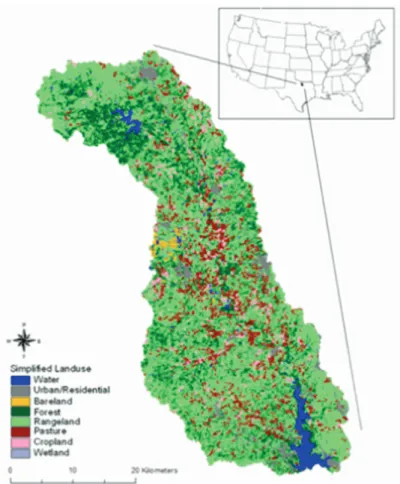
Eagle Mountain watershed, the total area of 2,230 km

, is located in northern Texas, USA (Figure 1). The Eagle Mountain Reservoir was constructed in 1932 and has served as a fresh water supply to the Dallas metropolitan area in northern Texas. The annual average rainfall in this watershed is 894 mm and average annual temperature is 26.5 (average high) and 14.3 (average low) degree Celsius. The watershed is a typical agricultural watershed and the major landuse of the watershed is rangeland, which takes 58.5% of the entire watershed (Figure 1 and Table 2).

National Elevation Dataset (NED) at 30 meter resolution was obtained from USDA-NRCS (United States Department of Agriculture - Natural Resources Conservation Service) Data Gateway web-site (http://datagateway.nrcs.usda.gov/) and used for delineating channel networks and subbasin. Elevation in the watershed ranges from 186 to 387 meter and channel flows from north to south and accumulates in the Eagle Mountain Reservoir. National Land Cover Dataset (NLCD) at also 30 meter resolution generated in 2001 was

Table 2. Landuse classification and percentages of each category

Landuse Percentage

Cropland 3.18%

Pasture 9.11%

Rangeland 58.50%

Urban 9.57%

Forest 17.42%

Water 2.18%

Wetland 0.04%

Total 100.0%

also obtained from NRCS Data Gateway and it was used in this study with enhancement of the dataset using aerial photographs taken in 2003 for urban area. Soil Survey Geographic (SSURGO) dataset, which is most detail dataset among currently available soil data, was obtained from the same web-site and used for soil information input. For weather data, minimum and maximum temperature and precipitation data was obtained from US National Climate Data Center (www.ucdc.gov) between 1969 and 2004 and total 13 weather stations were available within and around the watershed as shown in Figure 2.

NEXRAD (Next Generation Radar) dataset was also used to enhance observed precipitation data

from 1999. NEXRAD data is spatially distributed precipitation data, which is represented as 4 x 4 km grid and each pixel has a value for precipitation.

2) SWAT

SWAT (Soil and Water Assessment Tool) (Arnold et al., 1998) is a spatially distributed and continuous hydrologic model. Distributed hydrologic models allow a basin to be subdivided into many smaller subbasins to incorporate spatial detail. Water yield and pollutant loads are calculated for each subbasin and then routed through a stream network to the basin outlet.

Figure 1. The location of Eagle Mountain watershed and landuse map

SWAT goes a step further with the concept of Hydrologic Response Units (HRUs). In SWAT, a single subbasin can be further divided into areas with unique combinations of soil and land use, referred to as HRUs. ArcSWAT, which runs the SWAT model using ArcGIS interface developed by ERSI Inc., uses GIS (Geographic Information System) dataset to delineate watershed boundaries and channels, to input landuse and soil information, and to analyze results in various spatial and temporal scales. In this study, SWAT version 2005 was used.

3) Description of Previous Works

(1) Model Set Up

SWAT 2005 automatically delineated subbasins within the watershed using DEM and a contributing area definition threshold of 500 ha.

SWAT used landuse and soil information for

spatial variation in the watershed. The total

number of subbasins created by model was 150

and they are shown in Figure 3. There were

some subbasins partially submerged by the

reservoir and the area under the water in each

subbasin was calculated and accounted for the

effects of submergence in main channel inputs

(channel erodibility and channel cover were set

to “0.0”). SWAT simulated the land cover for these submerged areas as water.

SWAT’s input interface divided each subbasin into HRUs with unique soil and land use combinations. The number of HRU’s within each subbasin was determined by: 1) creating an HRU for each land use that equaled or exceeded two percent of each subbasin’s area and 2) creating an HRU for each soil type that equaled or exceeded 10 percent of any of the land uses selected in 1). Using these thresholds, the interface created 1,516 HRUs within the watershed.

Eagle Mountain watershed contained a total of 14 Waste Water Treatment Plants (WWTPs) from each major city and they are distributed in the watershed as shown in Figure 2. Two of these WWTPs discharge directly into the reservoir.

WWTPs voluntarily collected weekly nutrient and flow data for one year, which provided point- source loading inputs. This weekly data was converted to monthly loadings for each WWTP and included in the model. The Eagle Mountain watershed contains a total of 56 inventory-sized dams, as defined by the Texas Commission on Environmental Quality (TCEQ) in the US. These include NRCS flood prevention dams, farm ponds and other privately owned dams. The physical properties of each pond such as surface area, storage, drainage area, and discharge rates for these dams were input into SWAT model to allow routing of runoff through the impoundments.

Four ponds were big enough to be simulated as reservoirs while the rest were simulated as small ponds.

(2) Model Calibration and Validation

Lee et al. (2010) has conducted model calibration and validation using SWAT for Eagle Mountain watershed. Modeling period was from 1969 to 2004 (36 years) including two years of model warm-up period. The model calibration

was conducted from 1991 to 2004 and validation was conducted from 1971 to 1989. The validation time period was earlier than the calibration period because the land cover data used in this study was from 2001. Therefore, it was better to calibrate the model for the period of time that included the year of the land cover dataset.

Flow observation from two USGS gauge stations (08043950 and 08044500), shown in Figure 3, was used for flow calibration.

The initial values of each parameter in the model were based on surveyed and estimated watershed characteristics, or model default values if unknown. The model calibration for flow was conducted by adjusting appropriate input parameters that affect surface runoff and baseflow including the runoff curve number, soil evaporation compensation factor, shallow aquifer storage, shallow aquifer re-evaporation and channel transmission loss. The adjustment of input parameters were continued until the simulated total flow approximately agreed to the measured flow.

Figure 4 shows the result of monthly accumulated flow during the calibration and validation. R2 for calibration period was 0.947 and that for validation period was 0.964. Nash- Sutcliffe model efficiency (Nash and Sutcliffe, 1970) for calibration period was 0.913 and that of validation period was 0.921. More detail flow, sediment, and nutrients calibration process is described in Lee et al. (2010).

The sediment survey was conducted by Allen

et al. (2006) from Baylor University in early 2006,

collecting sediment cores to estimate the average

density and thickness of sediment at the lake

bottom. Allen et al. also conducted a watershed

survey to identify stream segments with channel

erosion problems and to quantify channel erosion

using NRCS field assessment techniques such as

RAP-M (Rapid Assessment Point Method). Allen

et al. calculated sedimentation in the Eagle

Mountain Reservoir by averaging three historical surveys. They concluded that the sedimentation

rate of the lake was 376,000 metric tons per year.

The delta sediment density was 1.25 kg per cubic

Calibration

Monthly Statistics:

R²: 0 947 R²: 0.947 ME*: 0.913

Validation

Monthly Statistics:

R²: 0.964 ME: 0.921

Figure 3. Observation data collection for model calibration and validation. Two USGS gage stations, multiple low flow sampling points, and monitoring stations were used for model calibration. Number in each subbasin indicate subbasin ID

Figure 4. The result of accumulated monthly flow calibration and validation at 08044500 site (Lee et al., 2010)

* ME: Nash-Sutcliffe (Nash and Sutcliffe, 1970) model efficiency

meter, pro-delta sediment density was 0.33 kg per cubic meter and average density was 0.51 kg per cubic meter. Based on the lake sediment survey and the watershed survey, researchers estimated that the erosion rate within Eagle Mountain watershed was about 340,883 metric tons per year. Out of this total, channel erosion contributed about 110,144 metric tons per year (32.3%) while the remaining sediment (230,739 metric tons per year) came from overland erosion (Allen et al., 2006).

The TWDB (Texas Water Development Board) conducted the second sediment study in 2008 with more recent technology using a duel frequency method (TWDB, 2008). TWDB estimated the thickness of the reservoir’s post- impoundment sediment. The study used the most recent technology and measured with very fine resolution. Therefore, the measurement was adopted for this study with some adjustment with previous sediment research by Allen et al. (2006).

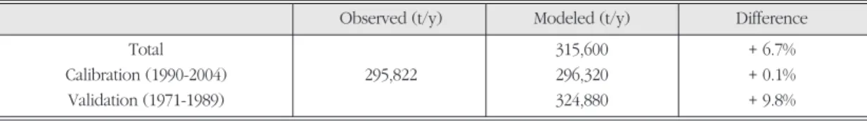
SWAT estimated sediments were compared with the observed sediment over a 34 years period from 1971 to 2004 and adjusted the appropriate input parameters until the estimated annual sediment load from overland and channel erosion were close to the measured load. Table 3 shows the result of sediment calibration and validation.

The average model estimation of sediment loading (315,500 tons per year) is close to the observation (295,822 tons per year) where the modeled sediment is little higher by 9.8% in the validation period.

Nutrient calibration consisted of two parts including calibration based on a low flow study, which was conducted August 18, 2004 and calibration using monitoring data (Figure 3). The low flow study was conducted in dry condition and the parameter adjustment was continued until the model estimation approximately agreed with observation. Then, the parameters were adjusted further against long-term monitoring station data, which included peak flows. WWTP data was only available for a year in 2002 from each WWTP, which was collected by the TRWD, and it was assumed that WWTP loadings at each facility were the same every year starting with the first year of operation. The percentage of each WWTP contribution in nutrients loadings to the reservoir was relatively low and the total loadings from all WWTPs were less than 2% of entire nutrient loadings to the reservoir.

The output from the calibration was compared with water quality data collected by TRWD (Tarrant Region Water District) from 1991 through 2004 in each major tributary (Ash, Derrett, Dosier, Walnut, and West Fork 4688 as shown in Figure 3). Figure 5 shows the result of validation. The bars and points in the graphs indicate the median, 25th percentile and 75th percentile of each day. While some sites disagreed between observed and measured data, the West Fork 4688 site, located at the end of the main channel before the lake entrance, agreed relatively well.

Table 3. Sediment calibration and validation at the reservoir

Observed (t/y) Modeled (t/y) Difference

Total 315,600 + 6.7%

Calibration (1990-2004) 295,822 296,320 + 0.1%

Validation (1971-1989) 324,880 + 9.8%

Source: Lee et al. (2010)

4) Biofuel Crop Implementation

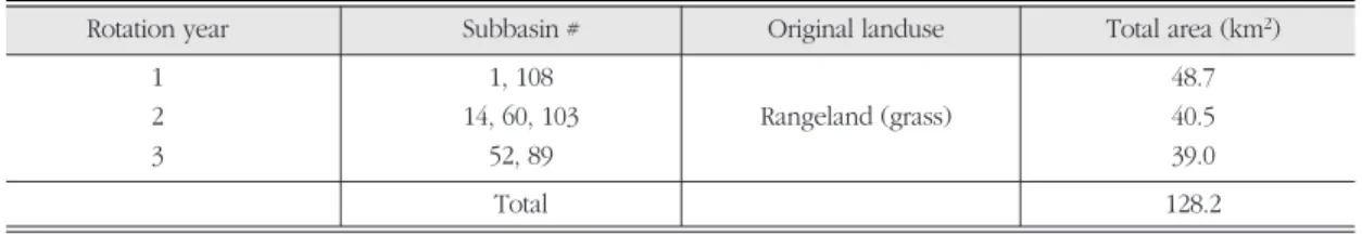
Switchgrass as a biofuel crop in this study was implemented in the model in the selected rangelands in Eagle Mountain watershed by implementing all required operation suggested by McLaughlin (2010). The total area of conversion was about 128 km2, which is about 5.4% of entire watershed. The location of switchgrass production in total seven watersheds was randomly selected and distributed watershed wide (Figure 6). The cropping system adopted a 3-year rotation that is consists of one year production and two years of fallow as suggested by McLaughlin (2010) as mentioned earlier.

Therefore, the total required area was approximately divided into three areas for rotation as shown in Table 4. Switchgrass was planted in subbasin 1 and 108 for rotation year 1, planted in subbasin 14, 60, 103 for rotation year

2, and planted in subbasin 52 and 89 for rotation year 3 (Figure 6, Table 4). The total area for each rotation year was 48.7, 40.5, and 39.0 km2 respectively. A detailed agricultural operation schedule is listed in Table 5, which is an example for the second year planting of switchgrass. The first year started with native grass as an initial plant followed by three tillage operation on October and November in the first year. Fertilizer was applied on December 1 with 269 kg/ha Nitrogen and 89 kg/ha Phosphorus. In the second year, switchgrass was planted on April 1 followed by two times of irrigation with 210 mm of water each. The total production of switchgrass was from 22 to 25 tons per hector, which was also estimated by model. For two years of fallow in each area, a natural grass (Johnsons grass) was planted to represent natural fallow without any agricultural operations. SWAT model was run with biofuel crop scenario from

Figure 5. Nutrient (Total Nitrogen and Total Phosphorous) validation at each monitoring site. Bar indicates range between 25% and 75% of all data and dot indicates a median value (Lee et al., 2010)

Table 4. The location and the area of switchgrass implementation by rotation years

Rotation year Subbasin # Original landuse Total area (km²)

1 1, 108 48.7

2 14, 60, 103 Rangeland (grass) 40.5

3 52, 89 39.0

Total 128.2

1969 to 2004 (36 years) and the first two years were not included in the result due to the model warm-up period.

5) Filter Strip Scenario

As a mitigation methodology for water quality degradation as the results of excessive nutrient loading by biofuel cropping, 30 meter wide filter strips were implemented in the subbasins as filter strip scenario where biofuel crops were planted.

In SWAT, a parameter called ‘FILTERW’in each HRU corresponding to converted croplands was changed from 0 to 30. The ‘FILTERW’means a filter strip width in unit of meter. Therefore, when the value of ‘FILTERW’is 30, it represents 30 meter wide filter strip in a particular HRU. The equation to calculate trapping efficiency for sediment and nutrients by filter strips is described (Neitsch et al., 2005) below.

Trap_ef

=0.367 · (Width

)

where, Trap

is the fraction of the constituent loading trapped by the filter strip, and Width

is the width of the filter strip in meter. Many researches (Bracmort et al., 2004; Renschler and

Lee, 2005; Lee et al., 2010; Pushpa et al., 2010) demonstrated the assessment of filter strips effectiveness using SWAT in their studies and they implemented the filter strips using above methodology and proved the reasonable estimation of the impacts of filter strips.

4. Results and Discussion

1) On-site impacts

Subbasins with biofuel crops scenario by converting from rangelands to croplands generate substantial amount of nutrients comparing to pre- biofuel crop (baseline). Figure 6 shows the yearly average on-site impacts for each subbasin where the amount of Total Nitrogen and Total Phosphorous was estimated at the outlet of each subbasin. Total Nitrogen and Total Phosphorous increased mainly because of the difference of fertilizer application between baseline with no fertilizer (rangeland) and biofuel crop scenario with tremendous amount of fertilizer (Table 1).

The three times of tillage operations and the twice of irrigations also played an important role

Year Date Operation Note

First 1/1 Native grass

10/1 Tillage

10/15 Tillage

11/1 Tillage

12/1 Fertilizer Application 269 kg/ha N, 89 kg/ha P

Second 4/1 Planting Switchgrass

4/15 Irrigation 210 mm

5/1 Irrigation 210 mm

9/1 Harvest 22-25 t/h production

Third 1/1 Native grass

to increase nutrient loading at the outlet. Table 6 summarizes the total amount of nutrients loadings for pre- and post-biofuel scenarios and the

percentage of increase in Total Nitrogen and Total Phosphorous in each subbasin. The Total Nitrogen and Total Phosphorous were increased

Table 6. The annual average increase of nutrients at each subbasin outlet. Baseline in the table indicates the scenario with pre-biofuel cropping and Biofuel in the table indicates the scenario with post-biofuel cropping

Subbasin Total Nitrogen (kg) Total Phosphorous (kg)

Baseline Biofuel Increase Baseline Biofuel Increase

1 4,851 60,862 1154.6% 475 3,150 563.2%

14 21,771 248,249 1040.3% 3,780 23,646 525.6%

52 47,995 167,761 249.5% 6,612 13,084 97.9%

60 12,817 109,316 752.9% 1,909 15,353 704.2%

89 15,612 193,084 1136.8% 2,260 23,864 955.9%

103 7,773 75,433 870.4% 1,589 19,014 1096.6%

108 15,038 169,520 1027.3% 3,577 32,635 812.4%

annually from about 250% to 1,150% and from about 100% to 1,100%, respectively.

2) Off-site impacts

The impacts of biofuel cropping at the reservoir were milder than on-site impacts due to the blending with flow from other subbasins. Table 7 summarizes the annual increase of nutrients at reservoir (the outlet of entire watershed). Total Nitrogen increased by 475 tons per hector annually (40.9%) with post-biofuel scenario while Total Phosphorous increased by 76.3 tons per hector annually (52.7%). Figure 7 compares the accumulative difference of each nutrient at reservoir between baseline and biofuel crop scenario for the modeling period (36 years). The graph indicates that the increase of nutrients

steadily increased at the rate of 40 to 50%

annually for both Total Nitrogen and Total Phosphorous.

3) Effectiveness of Filter Strips

The effectiveness of filter strips implemented in the subbasins with biofuel crop was evaluated at both on-sites (at the outlet of each subbasin) and off-site at reservoir (the outlet of entire watershed). Figure 8 illustrates the impacts of biofuel crop and filter strip in each subbasin that was selected for biofuel crop production. As shown in Figure 8, Total Nitrogen and Total Phosphorous dramatically increased due to the biofuel crops and decreased by filter strip in each subbasin. Table 8 shows annual average of Total Nitrogen and Total Phosphorous loading from each subbasin with biofuel crop scenario and filter strip scenario. The annual reduction rate by filter strip ranges from 58.0% to 67.9% for Total Nitrogen and from 57.7% to 68.2% for Total Phosphorous. It was found that 30 meter filter strip reduced the great portion of nutrients generated by biofuel crop production although there were still more nutrients loading compared to baseline.

Figure 7. Accumulated nutrients at reservoir during the modeling period (36 years) Table 7. Annual increase of nutrients at off-site (reservoir)

due to the production of biofuel crop

Total Nitrogen Total Phosphorous

(t/y) (t/y)

Baseline 1,162.4 144.7

With biofuel crop 1,637.4 221.0

Increase 40.9% 52.7%

The effectiveness of filter strip at reservoir, which can be an index of overall changes of water quality in the watershed, is shown in Table 9. The annual average Total Nitrogen loading from entire watershed was 1,162.4 tons per year

at baseline, increased to 1,637.4 t/y (+40.9%) by biofuel crop production, and then decreased to 1,171.1 t/y (-28.5%) by filter strip. The annual average Total Phosphorous loading from entire watershed also showed the similar pattern. It was

Table 8. The on-site effectiveness of filter strips by annual average of each nutrient. Biofuel in the table indicates post- biofuel cropping scenario and Filter Strips in the table indicates post-biofuel cropping with filter strips scenario

Subbasin Total Nitrogen (kg) Total Phosphorous (kg)

Biofuel Filter Strip Reduction Baseline Biofuel Reduction

1 60,862 24,344.8 60.1% 3,150 1,008.2 68.2%

14 248,249 79,439.7 67.9% 23,646 8,276.1 64.7%

52 167,761 63,749.2 62.3% 13,084 5,364.4 59.0%

60 109,316 37,167.4 65.8% 15,353 5,834.1 62.1%

89 193,084 59,856.0 69.2% 23,864 11,454.7 52.2%

103 75,433 31,682.9 58.0% 19,014 7,035.2 63.1%

108 169,520 61,027.2 64.1% 32,635 13,706.7 57.7%

Table 9. The effectiveness of filter strips at reservoir (off-site)

Total N (t/y) Increase/Reduce Total P (t/y) Increase/Reduce

Baseline 1,162.4 - 144.7 -

Biofuel crops 1,637.4 + 40.9% 221.0 + 52.7%

Filter strips 1,171.1 - 28.5% 156.0 -29.4 %

144.7 tons per year at baseline, increased to 221.0 t/y (+52.7%), and then decreased to 156.0 t/y (- 29.4%). Overall, the filter strips were effective to reduce nutrients loading and the amount of nutrients from entire watershed was close to baseline. Total Nitrogen loading increased by 8.7 t/y and Total Phosphorous increased by 11.3 t/y compared to the baseline.

5. Conclusion

The impacts of biofuel crop production on watershed and water quality was estimated using a pre- and post- scenario for long term period (36 years). The SWAT model was previously calibrated with observed data and was used as a baseline scenario. The economical and operational aspects of biofuel crop production were also previously investigated. Biofuel crop production requires tremendous amount of fertilizers, irrigation, and tillage operation to increase their productivity for cost effectiveness.

The biofuel crop scenario in the model estimated approximately 250% to 1,150% annual increase of Total Nitrogen and about 100% to 1,100% annual increase of Total Phosphorous at each subbasin outlet (on-site) where biofuel crop was implemented. For the watershed-wide level at the reservoir (off-site), the model estimated the annual increase of Total Nitrogen and Total Phosphorous by 40 to 50% comparing to the baseline.

A filter strip scenario was conducted by implementing filter strips in subbasins with biofuel crop production. The filter strips reduced nutrients annually at the outlet of each subbasin from 58.0% to 67.9% for Total Nitrogen and from 57.7% to 68.2% for Total Phosphorous, respectively. The effectiveness of filter strip at reservoir (watershed outlet) was the reduction of

28.5% for Total Nitrogen and the reduction of 29.4% of Total Phosphorous. Overall the 30 meter filter strip was effective to mitigate the increased nutrients due to the biofuel crops in this watershed.

Based on the results, the filter strips were effective to reduce the water quality degradation caused by biofuel crop production. To control nutrients including Total Nitrogen and Total Phosphorous is a key point to prevent on-site nutrient loadings to the waterbodies and off-site eutrophication in the reservoir. The biofuel production can be an important alternative energy source in Korea in terms of economical benefits. However, mitigation methodologies such as filter strips to protect environment and water quality are necessary to be considered before the biofuel production. The implementation of various types of BMPs as well as various widths of filter strips in the model based on the local conditions to estimate the impacts is helpful and recommended for watershed protection plan. This study provides an example and a guideline to assess the impacts on water quality by post-biofuel cropping and to consider the cost of biofuel production.

Reference

Allen, P. M., Dunbar, J. A., Prochnow, S., and Zygo, L., 2006, Cedar Creek: Stream Erosion and Reservoir Volume Evaluation, Baylor University and SDI Inc, Waco, TX.

Arnold, J. G., Srinivasan, R., Muttiah, R. S., and Williams, J. R., 1998, Large area hydrologic modeling and assessment, Part I: Model Development, Journal of the American Water Resources Association, 34, 73-89.

Bracmort, K.S., Engel, B.A. and Frankenberger, J.R., 2004, Evaluation of structural best management practices 20 years after installation: Black Creek

Watershed, Indiana, Journal of Soil and Water Conservation, 59(5), 659 - 667.

Dabney, S. M., 1998, Cover crop impacts on watershed hydrology, Journal of Soil and Water Conservation, 53, 207 - 213.

Dabney, S. M., Liua, Z., Lanec, M., Douglasc, J., Zhua, J., and Flanagan, D. C., 1999, Landscape benching from tillage erosion between grass hedges, Soil

& Tillage Research, 51, 219 - 231.

Dabney, S. M., 2003, Erosion control, vegetative, in B. A.

Stewart and T. A. Howell (ed.), Encyclopedia of Water Science, Marcel Dekker, New York, NY.

Dunne, T. and Leopold, L. B., 1978, Water in Environment Planning, W. H. Freeman and Company.

Energy Information Administration, 1993, State Energy Data Report. Consumption estimates, US Government Printing Office, Washington, D.C.

Flanagan, D. C., Foster, G. R., Neibling, W. H., and Burt, J. P., 1989, Simplified equations for filter strip design, Transaction of American Society of Agricultural Engineers, 32, 2001 - 2007.

Foster, G. R., 1982, Modeling the erosion process, in Haan, C. T. (ed.), Hydrologic modeling of small watersheds. Ameircan Society of Agricultural Engineeing Monograph No. 5, St. Joseph, MI.

Jin, C. X., Dabney, S. M., and Romkens, M.J., 2002, Trapped Mulch Increases Sediment Removal by Vegetative Filter Strips: a Flume Study, Transaction of American Society of Agricultural Engineers, 45, 929 - 939.

Lee, T., Rister, M. E., Narasimhan, B., Srinivasan, R., Andrew, D., and Ernst, M.R., 2010, Evaluation and spatially distributed analyses of proposed cost-effective BMPs for reducing phosphorous level in Cedar Creek Reservoir, Texas, Transaction of American Society of Agricultural Engineers, 53, 1619 - 1627.

Lee, T., Narasimhan, B., White, M., Wang, S., Tuppad, P., and Srinivasan, R., 2010, Trinity River Basin Environmental Restoration Initiative - Eagle Mountain Watershed, Tarrant Regional Water District, the Spatial Sciences Laboratory, and Texas AgriLife Research, Dallas, TX USA.

Mclaughlin, W. A., 2010, The economic and financial

implication of supplying a bioenergy conversion facility with Cellulosic biomass feedstocks, Unpublished Master Thesis, Texas A&M University, College Station, TX.

Nash, J. E. and Sutcliffe, J. V., 1970, River flow forecasting through conceptual models: Part I - A discussion of principles, Journal of Hydrology, 10, 282 - 190.

Neitsch, S. L., Arnold, J. G., Kiniry, J. R., Srinivasan, R., and Williams, J. R., 2005, Soil and Water Assessment Tool - Theoretical Document, Grassland, Soil and Water Research Laboratory, and Blackland Research Center, USDA-ARS, Temple, TX.

Novotny, V. and H. Olem., 1994, Water Quality:

Prevention, Identification, and Management of Diffuse Pollution, Van Nostrand Reinhold, New York, NY.

Pushpa, T., Douglas-Mankin, K.R., McVay, K.A., 2010, Strategic targeting of cropland management using watershed modeling, Agricultural Engineering International: CIGR Journal, 12(3), 12 - 24.

Renschler, S.C. and Lee, T., 2005, Spatially distributed assessment of short- and long-term impacts of multiple best management practices in agricultural watersheds, Journal of Soil and Water Conservation, 60(6), 546 - 556.

Römkens, M. J. M., Prasad, S. N., and Whisler, F. D., 1990, Surface sealing and infiltration, in Anderson, M. G. and Burt, T. P. (ed.), Process studies in hillslope hydrology, John Wiley and Sons, Ltd.

Syversen, N., Øygarden, L., and Salbu, B., 2001, Cesium- 134 as a tracer to study particle transport processes within a small catchment with a buffer zone, Journal of Environmental Quality, 30, 1771 -1783.

Thompson, A. M., Wilson, B. N., and Hansen, B. J., 2004, Shear stress partitioning for idealized vegetated surfaces, Transactions of American Society of Agricultural Engineers, 47, 701 - 709.

Tomlin, A. D., Shipitalo, M. J., Edwards, W. M., and Protz, R., 1995, Earthworms and their influence on soil structure and infiltration, in Hendrix, P.F.

(ed.), Earthworm Ecology and Biogeography in North America, Lewis Publication, Boca Raton, FL.

TWDB, 2008, Volumetric and sedimentation survey of Eagle Mountain Lake, Texas Water Development Board Report, Austin, TX.

USDA-NRCS, 1999, National Handbook of Conservation Practices, The US Department of Agriculture - Natural Resources Conservation Service, Washington, DC.

Virtus Energy Research Associates, 1995, Texas renewable energy resource assessment: Survey,

Overview & Recommendations, Report for the Texas Sustainable Energy Development Council, Austin, TX.

Correspondence: Taesoo Lee, 1500 Research Parkway, Suite B230, College Station, TX, 77843, USA, e-mail: taesoo@tamu.

edu, phone: 1-979-820-3215.

교신: 이태수, 이메일: [email protected], 전화: 1-979-820- 3215

Received January 28, 2011 Revised February 25, 2011 Accepted February 26, 2011