위상 민감도를 이용한 초탄성 비선형 구조의 레벨셋 기반 위상 및 형상 최적설계
김 민 근1․하 승 현2․조 선 호3†
1삼성중공업 풍력발전사업부, 2존스홉킨스대학교 토목공학과, 3서울대학교 조선해양공학과
Level Set Based Topological Shape Optimization of Hyper-elastic Nonlinear Structures using Topological Derivatives
Min-Geun Kim1, Seung-Hyun Ha2 and Seonho Cho3†
1WTG development team1, Samsung Heavy Industries, Geouje, 656-813, Republic of Korea
2Department of Civil Engineering, Jones Hopkins University, Baltimore, MD 21218, USA
3Department of Naval Architecture and Ocean Engineering, Seoul National University, Seoul, 151-744, Republic of Korea
Abstract
A level set based topological shape optimization method for nonlinear structure considering hyper-elastic problems is developed.
To relieve significant convergence difficulty in topology optimization of nonlinear structure due to inaccurate tangent stiffness which comes from material penalization of whole domain, explicit boundary for exact tangent stiffness is used by taking advantage of level set function for arbitrary boundary shape. For given arbitrary boundary which is represented by level set function, a Delaunay triangulation scheme is used for current structure discretization instead of using implicit fixed grid. The required velocity field in the actual domain to update the level set equation is determined from the descent direction of Lagrangian derived from optimality conditions. The velocity field outside the actual domain is determined through a velocity extension scheme based on the method suggested by Adalsteinsson and Sethian(1999). The topological derivatives are incorporated into the level set based framework to enable to create holes whenever and wherever necessary during the optimization.
Keywords : topological shape optimization, level set method, topological derivatives, hyper-elastic material, adjoint variable method, velocity extension scheme
†Corresponding author:
Tel: +82-2-880-7322; E-mail: [email protected] Received November 19 2012; Revised November 28 2012;
Accepted December 1 2012
Ⓒ 2012 by Computational Structural Engineering Institute of Korea
This is an Open-Access article distributed under the terms of the Creative Commons Attribution Non-Commercial License(http://creativecommons.
org/licenses/by-nc/3.0) which permits unrestricted non-commercial use, distribution, and reproduction in any medium, provided the original work is properly cited.
1. Introduction
In topology optimization fields, Bendsøe and Kikuchi(1988) introduced the homogenization method with by microscopic voids. Nowadays, the density approach such as solid isotropic materials with penalization(SIMP) method(Bendsøe and Sigmund, 2003) is generally utilized due to its simple imple- mentation compared with the homogenization method.
However, in SIMP method, lower density region causes unrealistic deformation especially in non-linear
structures. This phenomenon is well known as convergence difficulty problem which is actively discussed topics in non-linear analysis(Buhl et al., 2000). The convergence difficulty is due to relatively sparse materials exposed to the stress concentration.
For the non-linear analysis, incremental iterative schemes are usually preferred and the results from the previous steps are again used to proceed to the following incremental steps. Therefore, if unrealistic deformation from the previous steps in used, it may result in the convergence difficulty. Cho and Jung
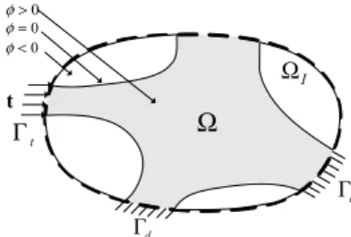
Ω
>0 φ
<0 φ=0 φ
Γd
Γt
t
ΩI
Γd
Fig. 1 Design domain and level set function (2003) developed an alternative method by using a
topology optimization method for displacement-loaded systems to resolve this convergence difficulty.
Since Osher and Sethian(1988) have devised a level set method for numerically tracking fronts and free boundaries, a level set method is introduced to the structural optimization problems. Wang et al.
(2003) developed a numerical procedure for topology optimization and represent the structural boundary using the level set model that is embedded in a higher dimensional scalar function. Allaire et al.
(2004) described a new implementation of a level set method for shape optimization. They considered the compliance and target displacement objectives.
Kwak and Cho(2005) applied level set optimization approach to the geometrically nonlinear structures in total Lagrangian formulation. The algorithm creates no holes inside the domain and converges to a local minimum which strongly depends on the initial topology.
In conventional shape optimization using a level set method, a kind of material penalization such as an initial reference domain(Wang et al., 2003) or an ersatz material(Allaire et al., 2004) is used to prevent from a singular problem, and these approa- ches cause the convergence difficulty problem again for non-linear analysis due to inaccurate stiffness.
Especially, a large strain is induced in a large deformation problem such as hyper-elastic material, and sometimes it causes an ill-conditioned tangent stiffness matrix.
In this research, a topological shape optimization method of hyper-elastic material is developed using level set methods. To prevent converence difficulty, actual boundary determined from the level set function is utilized in Lagrangian framework instead of implicit boundary representation. A Delaunay triangulation scheme(Persson and Strang, 2004) is used for the actual domain and an analysis for response and sensitivity is done within an actual domain without any material penalization techniques. The normal velocity which is used to update level set function is obtained from the sensitivity analysis
using adjoint variable method(Allaire et al., 2004;
Wang et al., 2003). Even if Newton-Rhapson iteration method is used in response analysis, the convergent tangent operator, obtained from this scheme, is directly used in solving the linear adjoint equation.
Since an analysis is done only in actual domain, the necessary normal velocity of domain outside for boundary propagation is obtained using velocity extension method(Adalsteinsson and Sethian, 1999).
The topological derivatives are incorporated into the level set based framework to enable to create holes whenever and wherever necessary during the optimi- zation.
2. Level set method
Let Ω⊂Rd be a bounded open domain with a smooth boundary Γ. The boundary Γ is composed of displacement boundary and traction boundary , and these boundaries have a relation as ∩ ∅. Imagine the boundary Γ moves in the direction normal to its boundary.
To derive the equation of moving boundary as time evolves, we embed this propagating boundary as the zero level set φ of a (d+1)-dimensional function
) , ( kφ
Φ . Given a closed d-dimensional hyper-surface
Γ, the implicit moving boundary is represented by the level set function φ
Ω Ω
∈ Γ
∈ Ω
∈
⎪⎩
⎪⎨
⎧
Γ
− Γ +
=
\ )
, (
0 ) , ( ) (
x I
x x x
x x
ζ ζ
φ (1)
where ζ(x,Γ) is a signed distance from a point x to
the boundary Γ . Ω is a fixed domain that includes I
all the admissible domain Ω. An outward unit vector n normal to the boundary Γ and a curvature H are obtained by
φ φ
∇
−∇
=
n , ⎟⎟
⎠
⎞
⎜⎜
⎝
⎛
∇
⋅ ∇
−∇
=
=divn φφ
H (2)
For the evolution of boundaries, we need to solve the Hamilton-Jacobi type partial differential equation (Osher and Sethian, 1988) as
τ φ φ = ∇
∂
∂
VN (3)
where VN is a normal velocity field determined from the design sensitivity analysis.
3. Response analysis for hyper-elasticity
The modified form of energy density function for the Mooney-Rivlin model is defined as
( 1 2 3) 10 1 01 2 ( 3 1)2
2 ) 1 3 ( ) 3 ( ,
,J J =A J − +A J − + J − J
W κ (4)
where A10 and A01 are material constants and κ is bulk modulus. Define J1, J2 and J3 as
( )
3 1/3 1 1=I I −J , J2=I2
( )
I3 −2/3, J3=( )
I31/2 (5)where I , 1 I , 2 I are the first, second, and third 3
invariants of the Cauchy-Green deformation tensor.
The abstract form of variational equation is
) ( ) ,
(z z =l z
a , for all z∈Z (6)
where z,z, and Z are the displacement, virtual displacement, and variational space which satisfies the essential boundary conditions, respectively. Defining the strain energy form a( zz, ) and load form l(z) as
Ω
≡
∫
Ωd0
)
; ( ) ( )
,
(z z 0 Sij z ij z z
a ε)
Ω
=
∫
Ωd0
)
; ( )
0 cijklεkl(zε)ij z z (7)
and
R z
t z
b
t i i i
i Ω+ Γ≡
≡
∫
Ω∫
Γ0
0 d
d )
(z 0 0
l (8)
where Sij(z), ε)ij( zz; ), b , and i ti are the second Piola- Kirchhoff stress tensor, virtual Green-Lagrange strain tensor, body force intensity, and surface traction, respectively. 0Ω and 0Γt are the structural domain and traction boundary at initial configuration, respectively. The Green-Lagrange and virtual strain tensors are given by
⎟⎟
⎠
⎞
⎜⎜
⎝
⎛
∂
∂
∂ + ∂
∂ + ∂
∂
= ∂
j m i m i j j ij i
x z x z x z x z
0 0 0
2 0
) 1
ε (z (9)
and
⎟⎟
⎠
⎞
⎜⎜
⎝
⎛
∂
∂
∂ + ∂
∂
∂
∂ + ∂
∂ + ∂
∂
= ∂
j m i m j m i m i j j
ij i x
z x z x z x z x z x z
0 0 0 0 0
2 0
) 1
; ( zz
ε) (10)
The material response tensor is defined as
kl ij kl ij ijkl
S W
c ε ∂ε ∂ε
= ∂
∂
=∂ 2 (11)
where is energy density function. Since the strain energy form is nonlinear in its argument z, Equation (6) cannot be solved directly. In this paper, an incremental-iterative scheme is adopted to solve the nonlinear system of equations. The external load is gradually increased and the solution of each load step is sought from the previous equilibrium solution.
At configuration (+1), the solution is decomposed into the solution at configuration () and the incre- ment as
z z z= +Δ
+ n
n 1 (12)
At current configuration (+1), the equilibrium equation is written as
R z
t z
b S
n i i n i
i n n ij n ij
t
1 0 1 0
1 0 1 1
d d
d )
; ( ) (
0 0
0
+ Γ
+ Ω
+ Ω
+ +
≡ Γ +
Ω
=
Ω
∫
∫
∫
zε) z z(13)
We can write a linearized strain energy form and
(a) Original domain (b) Topological varation (c) Shape variation Fig. 2 Variation domains
a load form for hyperelastic nonlinear structures in total Lagrangian framework as
)
; ( ) ,
;
(nz z z * nz z
a∗ Δ =l , for all z∈Z (14)
where
∫
∫
Ω Ω
∗
Ω Δ
+
Ω Δ
≡ Δ
0 0
0 0
d )
; ( )
; (
d )
; ( ) ( )
,
; (
z z z z
z z z z
z z
n ij n kl ijkl
ij n ij n
c S a
ε ε
η ) )
)
(15)
∫Ω
+ − Ω
≡ 1 0 0
*(nz;z) n R Sij(nz)ε)ij(nz;z)d
l (16)
and linearized strain term is
) 2(
) 1
;
( m,i m,j m,j m,i
ij Δ zz ≡ Δz z +Δz z
η) (17)
4. Design sensitivity analysis
4.1 Shape derivative
Using Equation (6), define a Lagrangian for compliance at configuration (+1) and the correspon- ding adjoint equation as
∫
∫
∫
Ω+ Γ
+ + Ω
+ +
+ = 0 ⋅ Ω+ 0 ⋅ Γ+ 0 ⋅ Ω
0 1 0
1 1 0
1 1 1 , )
( d d d
Ln n n n n n
t
λ b z
t z
b λ
z
∫
∫
Ω+ + Γ
+ ⋅ Γ− Ω
+ 0 n 1t λd0 0 cijkl kl(n 1z) ij(n 1z,λ)d0
t
ε
ε ) (18)
where λ is the solution of the following adjoint equation as
∫
∫
Γ+ Ω
+ ⋅ Ω+ ⋅ Γ
=
t
d
a(λ,λ) 0 n 1bλ0 0 n 1t λ 0 (19)
Taking the shape derivative of Equation (18) in the direction of V, we have the following expression Ha and Cho, 2007) as
( )
[ {
∫
Ω+ + + +
+ , )= 0 ∇⋅ ⋅( + )+ ⋅∇( + )⋅
(n1zλ n1b n1z λ n1t n1z λ n L&
(
⋅ +)
−} ]
Ω+κ n+1t(n+1z λ) cijklεkl(n+1z)ε)ij(n+1z,λ)Vd0
{ }
∫
Ω+ Ω
Π
⋅
∇
= 0 (n1z,λ)Vd0 (20)
4.2 Topological derivative
Consider a two-dimensional problem for simplicity
as shown in Fig. 2. Let Ω⊂R2 be an original domain without holes (a). Its boundary is denoted by
N
D∪Γ
Γ
=
Γ (Γ : Dirichlet; D Γ : Neumann). Also, let N ρ
ρ =Ω\ω
Ω be an open domain with holes (b). Its boundary is denoted by Γρ=Γ∪∂ωρ. ωρ=ωρ∪∂ωρ is a complete circular domain of radius ρ(xˆ) centered at the point xˆ∈Ω.
Let Ωρ+τ =Ω\ωρ+τ be a perturbed domain (c). Its boundary is denoted by Γρ+τ =Γ∪∂ωρ+τ. ωρ+τ =ωρ+τ
τ
ωρ+
∂
∪ is a complete circular domain of radius ˆ)
( ˆ) (x τδρx
ρ + centered at the point xˆ∈Ω. When a hole is created during the topology optimization, it is impossible to build a homeomorphic map between the domains Ω and Ωρ. Using asymptotical regulariza tion concept, the topological variation ψT′(xˆ) is defined as the limit of shape variation when the radius of the holeρ(xˆ) approaches to zero.
0 0
0
) ( ) lim (
lim ˆ)
( + =
+ +
→
→ ⎪⎭
⎪⎬
⎫
⎪⎩
⎪⎨
⎧ ΨΩ −ΨΩ
=
′ ρτ τ
τ ρ
ρ τ
ρ τ
ρ δω
ψT x ω
ρ ρ
ρ τ
ρ ψ δω ψ δω
ω ( ) (ˆ)
lim 1
,
0 &S x ≡ &T x
⎪⎭
⎪⎬
⎫
⎪⎩
⎪⎨
=⎧→ (21)
where ⋅ denotes the negative function of Lebesque measure of the set. ψ&T(xˆ) denotes the topological derivative. To calculate the topological derivative from the concept above, we need the shape derivative around the ball centered at xˆ. To this end, the perturbation is made only on the boundary of hole that has homogenous Neumann boundary condition as
ωρ 0 1
1 ⋅+ =0 ∂
+ n on
n S n .
The Lagrangian for the instantaneous compliance in the domain 0Ωρ=0Ω\0ωρ has the same form as
Equation (20). Note that since only the boundary of hole is perturbed, the design velocity vanishes on the other boundary. Using the following relations,
Vn
πρ πρδρ ω
δ ρ =2 =−2 , and
∫
∫ + = =− ∂ ∂
−
=
+τ ρ
ρ ω ρ
ω ρττ
ρ τ τ ω ω
ω d Vn
d d
, 0 (22)
The topological variation for the instantaneous compliance in Equation (18) is rewritten, in the absence of body force for the simplicity of problem as
n n
n n
n
T Vd V
V
L πρ
ω ρ
ρ
ω ρ ρ ρ
ω ρ
ρ 1 ( , ) 2
lim ˆ) )(
,
( 0
0
0 1
0 0 1
⎪⎭
⎪⎬
⎫
⎪⎩
⎪⎨
⎧
Γ
∂ Π
′ =
∫
∫
∂+
∂
→
+zλ x z λ
(23)
To calculate this limit to obtain the final expression of the topological derivative, we use an asymptotic analysis to obtain the behavior of solution S(n+1zρ)when ρ→0. This behavior may be obtained from the analytical solution for a stress distribution around a circular void in two-dimensional elastic body in polar coordinates(Novotny et al., 2000). Finally, the topological variation is expressed as
ˆ) )(
, ( 2 ˆ) )(
,
(+1zλ x =− Σ +1zλ x
′ n n n
T V
L πρ (24)
The topological variation of compliance is always positive when the hole is created since the topological derivative and the velocity Vn on the boundary of hole is always negative. This means that the comp- liance increases when the hole is created.
5. Topological shape optimization
5.1 Optimization formulation
The objective of topological shape optimization is to find an optimal layout that minimizes the instan- taneous compliance of the system under prescribed loadings. Considering the domain and boundary before nucleation, the topological shape optimization
problem is stated as
Min.
∫ ∫
Γ+ + Ω
+
+ ⋅ Ω+ ⋅ Γ
=
N
d
d n n
n n
0 0
0 1 1 0
1
1b z t z
ψ (25)
Subject to 0 max
0d M
m=∫Ω Ω≤ (26)
where Mmax is an allowable volume. The velocity field V(x) defines the propagation speed of all level sets along the outward normal direction. The velocity should be determined such that it reduces the instantaneous compliance while satisfying the requirement of allowable material volume. Thus, the following Lagranian is defined for the constraint optimization problem,
{
2 max}
) , ,
( s = + m+s −M
Λτ μ ψ μ (27)
where s and are a slack variable to convert the inequality constraint to the equality one, and a Lagrange multiplier, respectively.
5.2 Computation of design velocity
Using the Kuhn-Tucker optimality condition, the following is obtained(Allaire et al., 2004),
{
( , )}
0) , , (
0
0 1
0
= Ω +
Π
⋅
∇
Λ =∫Ω
+
=
d d V
s d
n
n zλ ξ n
τξ τ
τ (28)
where
⎪⎩
⎪⎨
⎧
≥ Ω
<
= Ω
∫ ∫
Ω Ω
max 0
max 0
0 0
if
if 0
M d
M d
ξ μ (29)
Then, we can take the normal velocity V as the n
descent direction as
{
Π +ξ}
−
= (n+1z,λ)
Vn (30)
where the Lagrange multiplier ξ is defined from shape derivative of volume constraint
{ }
∫ ∫
Ω Ω
+
Ω
⋅
∇
Ω Π
⋅
− ∇
=
0 0
0 0 1 , ) (
d
n d n
n λ
ξ z (31)
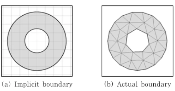
(a) Implicit boundary (b) Actual boundary Fig. 3 Delaunay triangulation
Fig. 4 Velocity extension domain inside (domain inside velocity interpolation, Equation (35)) 5.3 Optimization formulation
Equation (31) implies the averaged internal energy around the boundary. Using the topological derivative from Equations (21), (24) and (27), the following nucleation criterion can be obtained.
ξ μ
τμ ψ τ
τρ = + =−Σ +
Λ +
=→ ( , )(ˆ)
) , ,
( 1
00 T mT n z λ x
d s
d & & (32)
which implies the difference of compliance sensitivity between topological and shape variations. To ensure the decrease of compliance by the nucleation of holes, Equation (32) should be negative. Thus, the point ˆx can be possible nucleation points if the following criterion is negative
ε ξ− + Σ
−
=
Θ(xˆ) (n+1z,λ)(xˆ) (33)
where ε is a specified value that can control the number of nucleation holes. After nucleation of holes, it is necessary that the level set function must keep the signed distance properties(Wang et al., 2003).
Therefore, following reinitialization process is perfor- med such that the distance function at points x
around ˆx satisfies the following relation:
) ˆ) ( ), , ( min(
) ,
( τ φ τ 2 ρ
φ x = x x−x − (34)
6. Unstructured mesh generation and design velocity extension
6.1 Delaunay triangulation scheme
During the structural optimization process, the design domain keeps changing as the boundary evolves according to the time integration of the level set function. To handle the changing domains, numerical techniques such as initial reference domain or ersatz material are usually employed in the conventional level set based shape optimization.(Fig. 3(a)) To relieve the convergence difficulty, a re-meshing scheme is employed for the actual domain which is deter-
mined from the obtained level set functions.(Fig.
3(b)) Using the Delaunay triangulation, the actual domain is discretized into numbers of triangle elements.
6.2 Design velocity extension
In the level set method, the Hamilton-Jacobi equation for the level set function is solved at the fixed grid points in the initial domain, including outside the actual domain. To solve the H-J equation, velocity fields need to be given at least in the narrow band region. Therefore, some interpolation and extrapola- tion schemes are necessary to obtain the required velocity field in the level set method.
In the domain inside, the unstructured meshes for the response analysis generally do not coincide with the fixed grids for the level set method. Therefore, we need to interpolate the normal velocity at a fixed grid point using a distance-weighted average(Fig. 4) such as
∑
∑
=
i i
i i i
grid V d
V d1 1
(35)
where di and Vi are the distance between the fixed grid point to each unstructured mesh point and the
Fig. 5 Velocity extension domain outside (domain outside velocity interpolation, Equation (36))
Fig. 6 Boundary and loading conditions
Fig. 7 Convergence difficulty
(0) (0)
(29) (10)
(247) (80)
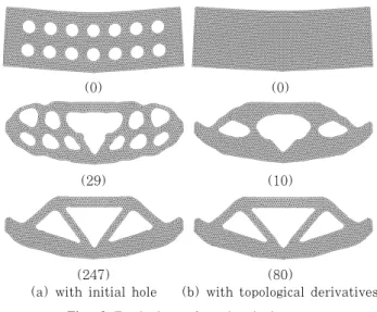
(a) with initial hole (b) with topological derivatives Fig. 8 Evolution of optimal shapes
given normal velocity obtained from the sensitivity analysis at each mesh point, respectively.
The velocity domain outside is based on the Adals- teinsson and Sethian(1999; Fig. 5). To maintain the signed distance property, the velocity fields are extrapolated using the following relation,
=0
∇
⋅
∇VN φ (36)
7. Numerical examples
7.1 Simply supported plate
A simply supported plate is subject to a vertical loading of 2×10⁻² at the center of lower side(Fig. 6). The dimension of the initial model is 1.8m long, 0.6m wide and 0.01m thick. The material follows Mooney-Rivlin hyper-elastic model with the properties: 75, 25, and κ=104. The model is composed of 3,325 grids for level set method. The objective optimization is to minimze compliance for given force with 40% volume fraction constraint.
Fig. 7 shows the convergence difficulty in geome- trical nonlinear problems using the implicit boun- dary. The red part is filled with solid homogeneous materials and blue one with void sparse materials. In the sparse material region, severe mesh distortion occurs due to the extreme material distribution at the near of side boundaries.
However, this numerical convergence difficulty can be avoided if the void sparse materials are eliminated by using explicit boundary through discretization of actual domain as shown in Fig. 8.
Fig. 8 shows the evolution of the optimal shapes for
the shape optimization with initial holes(without topological derivatives, Fig. 8(a) : case (a)) and for the topological shape optimization with topological derivatives and no initial holes (Fig. 8(b) : case (b)) for given boundary condition in Fig. 6. Accor- ding to the corresponding normal velocity field, the explicit boundary determined from the velocity extension scheme evolves to the optimal shape.
Using the topological derivative, nucleation is made whenever and wherever necessary depending on the indicator function given in Equation (33). Fig. 9 shows the results of topological derivatives at initial step, and topological shape change is occurred based on Equation (33). In Table 1, even though the objective functions obtained from cases (a) and (b) are almost same, the necessary iterations for the whole optimization and the satisfaction of
Case Number of Iterations
Iterations for Volume Constraint
Objective Function
(a) 247 96 9.377E-3
(b) 80 33 9.373E-3
Table 1 Comparison of optimization results Fig. 9 Topological derivative values
0 1 0 2 0 3 0 4 0 5 0 6 0 7 0 8 0 9 0
0 50 100 150 200 250 300
Number of iterations
Volume fraction (%)
0 0.002 0.004 0.006 0.008 0.01 0.012
Volume fraction Compliance
Compliance
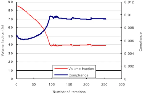
Fig. 10 with initial holes(shape variation only)
0 20 40 60 80 100 120
0 20 40 60 80 100
Nu mbe r of iterations
Volume Fraction (%)
0 0.002 0.004 0.006 0.008 0.01 0.012
Compliancece
V olume fr actio n C omp lia n ce
Fig. 11 with topological derivatives (shape and topological variations)
volume constraint in the case (b) are reduced to one-third of that in the case (a).
Topological derivatives make it possible to deter- mine the optimal position of nucleation of hole. Once topological variation occurs, that is, nucleation, the other variations are handled by successive shape variations. For the case (a), only shape variations are occurred for non-optimal hole position. Therefore, much more shape variations are needed when an arbitrary initial holes are given than when the optimal holes are determined by the topological derivatives(Kim et al., 2009). This shows that the topological shape variation with topological deriva- tives is more effective than shape variation methods.
Fig. 10 and Fig. 11 show the optimization history of case (a) and (b). Together with Table 1, we can notice that the developed method is very efficient.
Due to the volume constraint, the instantaneous- compliance functional is increasing until the volume
constraint, which is 40% of original one, is satisfied.
After that, the instantaneous compliance is mini- mized while holing the constraint. Small bumps in the instantaneous compliance are due to drastic topological changes such as merging and breaking of boundaries.
8. Conclusions
In this research, we performed level set based topological shape optimization for hyper-elastic problem.
To relieve convergence difficulty in nonlinear structure problem, we use the actual domain with the Dena- unay triangulation and a velocity extension scheme both inside and outside domain to integration Hamilton-Jacobi equation for update level set function. By using topological derivative concept, we can make holes in the domain wherever and when- ever we want. It can give us fast optimal shape independent of initial holes.
Acknowledgement
This research was supported by Basic Science Research Program through the National Research Foundation of Korea(NRF) funded by the Ministry of Education, Science and Technology(Grant Number 2010-18282). The support is gratefully acknowledged.
References
Adalsteinsson, D., Sethian, J.A. (1999) The Fast
요 지
초탄성을 고려한 비선형 구조의 레벨셋 기반 위상 및 형상 최적설계 방법을 개발하였다. 전체 영역에서 재료의 극단적인 불균형 분포로 기인하는 부정확한 접강성행렬(tangent stiffness matrix)로 인해, 비선형 문제의 위상 최적설계는 심각한 수 렴성의 어려움을 겪는다. 이를 해결하기 위해, 임의의 형상을 표현할 수 있는 레벨셋 방법의 장점을 이용하여 정확한 접강성 행렬을 구하기 위해 명시적인 경계(explicit boundary)를 이용하였다. 레벨셋 함수로 표현되는 임의의 영역을 암시적 고정 격 자(implicit fixed grid)를 이용하여 계산하는 것 대신에 명시적으로 그 영역을 이산화하기 위해 딜라우네이 삼각화 기법 (Delaunay triangulation scheme)을 이용하였다. 레벨셋 방정식을 풀기 위해 최적화 조건으로부터 라그란지안(Lagrangian;
목적함수)가 감소하는 방향이 되도록 속도장을 결정하였다. 실제 영역 바깥쪽 속도장은 Adalsteinsson와 Sethian(1999)가 제 안한 속도확장 기법을 이용하여 구하였다. 레벨셋 기반의 최적화 기법에 위상 민감도를 이용하여, 최적화 과정에서 원하는 시기와 위치에 위상 변화가 가능하도록 하였다.
핵심용어 : 위상 및 형상 최적화, 레벨셋 방법, 위상 민감도, 초탄성 재료, 보조변수 방법, 속도장 확장 기법 Construction of Extension Velocities in Level Set
Methods, Journal of Computational Physics, 148, pp.2~22.
Allaire, G., Jouve, F., Toader, A.M. (2004) Structural Optimization using Sensitivity Analysis and a Level-Set Method, Journal of Computational Physics, 194, pp.363∼393.
Bendso̸e, M.P., Kikuchi, N. (1988) Generating Optimal Topologies in Structural Design using a Homogenization Method, Computer Methods in Applied Mechanics and Engineering, 71, pp. 197∼
224.
Bendso̸e, M.P., Sigmund, O. (2003) Topology Optimi- zation: Theory, Methods and Applications, Springer- Verlag, Berlin, pp.370.
Buhl, T., Petersen, C.B.W., Sigmund, O. (2000) Stiffness Design of Geometrically Nonlinear Struc- tures using Topology Optimization, Structural Multi- disciplinary Optimization, 19, pp.93∼104.
Cho, S., Jung, H. (2003) Design Sensitivity Analysis and Topology Optimization of Displacement-Loaded Nonlinear Structures, Computer Methods in Applied Mechanics and Engineering, 192, pp.2539∼2553.
Ha, S.H, Cho, S. (2009) Level Set Based Topological Shape Optimization of Geometrically Nonlinear Structures using Unstructured Mesh, Computers &
Structures, 86, pp.1447∼1455.
Kim, M.G., Ha, S.H, Cho, S. (2009) Level Set-Based Topological Shape Optimization of Nonlinear Heat
Conduction Problems using Topological Derivatives, Mechanics Based Design of Structures and Mach- ines, 37, pp.550∼582.
Kwak, J., Cho, S. (2005) Topological Shape Optimi- zation of Geometrically Nonlinear Structures using Level Set Method, Computers & Structures, 83, pp.2257∼2268.
Mooney, M. (1940) A Theory of Large Elastic Defor- mation, Journal of Applied Physics, 11 pp.582∼
592.
Novotny, A.A., Feijoo, R.A., Taroco, E., Padra, C. (2000) Topological Sensitivity Analysis, Compu- tational Methods in Applied Mechanics and Engi- neering, 188 pp.713∼726.
Osher, S., Sethian, J.A. (1988) Front Propagating with Curvature Dependent Speed: Algorithms Based on Hamilton-Jacobi Formulations, Journal of Computational Physics, 79, pp.12∼49.
Persson, P., Strang, G. (2004) A Simple Mesh Henerator in Matlab, SIAM Review, 46(2), pp.329
∼345.
Sokolowski, J., Zochowski, A. (1999) A. On Topological Derivative in Shape Optimization, SIAM Journal of Control and Optimization, 37, 1251∼1272.
Wang, M.Y., Wang, X., Guo, D. (2003) A Level Set Method for Structural Topology Optimization, Computational Methods in Applied Mechanics and Engineering, 192, pp.227∼24.