1. Introduction
The remote sensing models for evapotranspiration estimation(ET) can be divided into three basic ways, (1)analytical solutions, (2)modeling approaches, and (3)semi-empirical and statistical methods(Moran and Jackson, 1991). Analytical methods calculate ET by combining remotely sensed spectral data with ground- based meteorological data.(Price, 1980, 1982; Jackson, 1985). Modeling approaches use to simulate the surface energy budget by solving numerical equations for heat
and mass transfer in combination with remotely sensed data and limited meteorological data(Carlson and Boland, 1978; Carlson et al., 1981; Taconet et al., 1986;
Soer, 1980; Gurney and Hall, 1983; Running et al., 1989). In the last method, the evapotranspiration is estimated from remotely sensed surface temperature based on a statistically established formula. This method has been suggested by Jackson et al. (1977).
All remote sensing methods can not estimate ET without a ground-based measurement. The semi- empirical method can estimate ET with three
Extension Test of Midday Apparent
Evapotranspiration toward Daily Value Using a Complete Remotely-Sensed Input
Kyung-Soo Han* and Young-Seup Kim**
CNRM/GMME/MATIS, Meteo-France, France*
Department of Satellite Information Sciences, Pukyong National University**
Abstract :The so-called B-method, a simplified surface energy budget, permits calculation of daily actual evapotranspiration (ET) using remotely sensed data, such as NOAA-AVHRR. Even if the use of satellite data allows estimation of the albedo and surface temperature, this model requires meteorological data measured at ground-level to obtain the other inputs. In addition, a difficulty may be occurred by the difference of temporal scales between the net radiation in daily scale and instantaneous measurement at midday of the surface and air temperatures because the data covered whole day are necessary to obtain accumulated daily net radiation. In order to solve these problems, this study attempted a modification of B-method through an extension of hourly ET value calculated using a complete instantaneous inputs. The estimation of the daily apparent ET from newly proposed system showed a root mean square error of 0.26 mm/day as compared the output obtained from the classical model. It is evident that this may offer more rapid estimation and reduced data volume.
Key Words :Evapotranspiration, AVHRR, B-method, Surface Temperature.
Received 20 March 2003; Accepted 15 July 2003.
variables(net solar radiation, surface temperature and air temperature), which can be obtained from satellite. But, the first and second methods still require the help of ground-based measurement for other parameters.
Remotely sensed actual ET(ET*, i.e., apparent ET) is usually derived from the surface energy budget in combination with the governing equations for water flux, sensible heat, and radiative energy exchange between the surface and the atmosphere(Carlson and Buffum, 1989).
The “B-method” of Jackson et al.(1977), further developed by Seguin and Itier(1983), and Carlson and Buffum (1989), is a typical simplification for remote sensing applications. This approach has two principal limitations. First, the use of satellite data allows estimation of the albedo and surface temperature while the models require ground-level measurements from meteorological stations to obtain the other variables necessary to calculate evapotranspiration. Although evapotranspiration can be estimated by this methodology, estimates that cover large areas cannot be provided, only local values around meteorological stations. It is evident that this information used may be locally precise, but the biases resulting from its extrapolation in space are often magnified, especially when the density of meteorological stations is low. In addition, many microphysical processes are grossly parameterized to capture their effects, with a minimum of computational expense, within the coarse resolution of the models. Therefore, there is a need for advanced techniques for the parameterization and reproduction of model inputs using remote-sensing data, in order to provide an image of the surface that is regularly resolved in space and time. Second limitation is the difference of temporal representativities between accumulated net radiation in daily scale and instantaneous measurement at midday of air and surface temperatures. In particular, the use of accumulated net radiation in daily scale using satellite data should suffer the infrequent coverage and
high costs, in addition to the high data volume.
In this study, we will overcome the problems resulted from the limitations using an estimation of extended ETd* from hourly ET* model based on the B-method with a remotely sensed Tavalue, witch is obtained by multiple statistic analysis using the digital elevation model, digital land use, and Tsas input parameters.
Finally the modified B-method proposed will be compared to its original model.
2. Study Area
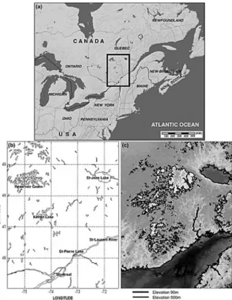
The study area was a zone corresponding to the western part of Quebec, Canada, located between 71.47˚
~ 75.65˚W and 45.03˚~ 49.74˚N(Fig. 1). This zone (Fig. 1(a) and (b)) covers an area of approximately 174,080km2. Fig. 1(c) shows the topography of the study area calculated using the Digital Elevation Model(DEM) from 1:25,000 scale topographic maps from Geomatics Canada with a contour interval of 30m.
Mountains higher than 500m are located along the river valley to the northwest, in the mid-eastern part of the study area, and in the region between the St. Jean Lake and the Gouin Reservoir. The study area consists of various surface types, including forest, agricultural regions, lakes, rivers, open land, and urban areas. All the data used in this research were collected in two periods of 1 to 10 June and 1 to 10 July 1997, which include the summer growing season and the peak of forest fire activity.
Two ecozones dominate the landscape in the study area: forest and agricultural regions. Forest covers 77%
of the study area. The agricultural region borders the St.
Lawrence River and the St. Jean Lake. Needle-leaf forests are distributed mainly in the northwestern part of the study area, while broad-leaf forest is widely distributed throughout the study region, except for agricultural areas. The mountainous areas have dense
vegetation cover. Six distinct land covers are present while urban areas and water surfaces are ignored:
needle-leaf forests (23.13%), broad-leaf forests (53.04%), open land (shrub(5.42%), grass (0.03%) and barren (0.15%)), and crop land (13.32%).
3. Data Set
Wind velocity(U) and air temperature(Ta) were obtained from surface meteorological instruments and recorded at 42 automated meteorological stations in three different regional networks. There were 11 Environment Canada stations, 9 stations in the POMMIER network of MAPAQ(Ministere de Agriculture, des Pecheries et de Alimentation du
Quebec), and 22 SOPEU(Societe de Protection des Forets contre le Feu) stations.
Visible and infrared satellite data are used in surface temperature(Ts) calculations. We used NOAA/AVHRR (National Oceanic and Atmospheric Administration/
Advanced Very High Resolution Radiometer) data from NOAA-12 and NOAA-14. The satellite data covered two periods(1~10 June and 1~10 July, 1997) and were obtained from Environment Canada. Channels 1~5 from the AVHRR are used. The horizontal spatial resolution of the data is about 1 km×1 km at nadir for all AVHRR channels. The radiance values for each channel are converted to several variables. Infrared AVHRR data have been processed to yield brightness temperatures, while the visible and near-infrared AVHRR data have been processed to yield reflectance,
Fig. 1. Maps of (a) eastern North America (b) enlarged study area(rectangle in (a)), and (c) its elevation: thick and thin lines indicate 90m and 500m contours, respectively.
which is used to calculate NDVI(Normalized Difference of Vegetation Index) and to detect cloud contamination.
4. Estimation of Tsand Ta
Remotely sensed actual ET* is derived from the surface energy budget in combination with the governing equations for water flux, sensible heat, and radiative energy exchange between the surface and the atmosphere, with assumption that the ground cover is homogeneous within each sensor footprints (pixels), as follows:
<LE> _<Rn> = _<H> = _r·Cr· (1) where <LE> is the latent heat flux, <H> is the sensible heat flux, <Rn> is the net radiation flux, r is the air density, Cris the specific heat of air at constant pressure, Tsand Taare surface and air temperatures, respectively, and rais the aerodynamic resistances.
The simplified B-method for remote sensing applications is as follows:
ETd*_Rnd= Bd·(Ts_Ta)i (2) where ETd*is expressed in mm/day, Rnd= <Rn>/l is the net radiation expressed in mm/day, l is the latent heat of vaporization, the subscripts d and i indicate daily and instantaneous at midday values, and Bdis the semiempirical coefficient.
The most important problems related to the accurate measurement of Tsfrom space are the elimination of atmospheric absorption and correction for emissivity.
Water vapor absorption can be eliminated by using two contemporaneous measurements at different wavelengths inside the atmospheric window 10.5
~12.5mm. This split-window technique has been successfully applied for sea surface measurements with AVHRR(Coll, et al., 1994). Split-window methods are frequently used, and take advantage of the different atmospheric characteristics in two adjacent spectral
bands in the infrared (around 11 and 12mm).
A simple extension of the split window technique for land surface temperature determination by Ulivieri et al.(1994) has been set up; it is theoretically possible to express Ts as a combination of the brightness temperatures in two spectrally adjacent channels, also separating the atmospheric absorption and the surface emittance effects if the total water vapour amount is less than 3.0g/cm3. This is a split window algorithm with the following form;
Ts= T4+ 1.8(T4_T5) + 48·(1 _e) _75·De (3) where T4and T5are the brightness temperature of channel 4 and 5, respectively, e is the mean emissivity (= (e4+ e5) /2), and De is the emissivity difference (= e4
_e5). This algorithm later was found to be accurate to 3K for a uniform tall grass prairie habitat in Kansas, when a constant emissivity was assumed(Cooper and Asrar, 1989).
Most remote sensing methods for estimating apparent ETd combine spectral data with ground-based meteorological data. This is a major drawback whenever the meteorological network is scarce, such as for this study. For such cases, the usefulness of satellite data is extended to the estimation of meteorological parameter, namely Ta*(Han, et al., 2003 a). A stepwise third-order polynomial multiple regression model has been semi- empirically proposed by Han et al.(2003 b and c) as follows;
Ta*= b0+ Sn
i=1bi·Fi (4)
where b0is a constant, biis the coefficient of i-th independent variable Fi, and n is the number of independent variables. Since the Ta values vary as a cubic function over the course of a day, the maximum degree of the polynomial was set to the third-order.
Consequently, 84 independent variables were first obtained from six input components. Using a stepwise method, a third-order polynomial multiple regression was established with 30 final independent variables that Ts_Ta
ra
are significant at the 0.05 level (Table 1). To optimize execution of the model, the units of the input variables are as follows: Ts (degrees), NDVI (0 ~ 1), digital elevation model (kilometres), local time (decimal), Julian-day/365 (0 ~ 1), and latitude (radians). For the estimated regression model, the value of coefficient of determination (R2) was 0.88 and RMSE between the estimated and measured Tavalues are 2.21˚C.
5. Original B-method System
Note that for the rest of the paper, in order to avoid confusion between the various time scales involved, the suffix d will identify daily values, h hourly values, m maximum values (taken as occurring at 13:00 LST), and i instantaneous values.
Daily B need to be evaluated in order to estimate daily apparent ET* from Eq. (2), where in this case Ts and Ta*are maximum daily value (taken as 13:00 LST).
The coefficient Bdvalues represent the slopes of the regressions between the terms (Ts- Tah) and (ETd- Rnd) in Eq. (2). The second term can be obtained by the energy balance equation of (1). The formulation of the coefficient B in Seguin and Itier (1983) method requires
the careful definition of the aerodynamic resistance ra. Above a plant canopy, the wind velocity within a neutral surface layer (zero heat flux) follows a logarithmic function of reference height (Stannard, 1993). In this study, ravalues are calculated following Monteith and Unsworth (1990);
ra= (5)
k2·U
where z is the height of the anemometer (=10m), z0is the surface roughness length (m), d is the zero plane displacement height (m), k is the Karman constant (=0.41), and U is the wind velocity (m/s). Table 2 is a look-up table of the plant descriptors h, z0and d used for each land covers (needle leaf forest, broadleaf forest, shrub land, cropland, grassland and barren land).
Therefore, (ET* - Rn) term in Eq. (2) is based on roughness length, zero-plane displacement, Ta, and wind speed. The values of Bdmainly vary according to z0: the slopes increase with decreasing the surface roughness length over same surface type. Least square results of B for each land cover classes are 0.08 for barren land, 0.11 for grass land, 0.14 for crop land, 0.17 for shrub land, 0.53 for broad leaf forest and 0.94 for needle leaf forest (Fig. 2). Theses values are in general agreement with the
[ln(z _d) ]2 z0 Table 1. Independent variables and coefficients of Taestimation model(Han et al., 2003 b).
Ta estimation, (n = 31)
Fi bi Fi bi Fi bi
b0= -333.62 F11= x4x5x1 b11= 2.35 F22= x33 b22= -0.01 F1= x13 b1= -0.0002 F12= x52x1 b12= -1.28 F23= x32x4 b23= 0.13 F2= x12x2 b2= -0.004 F13= x1 b13= 0.76 F24= x32 b24= 0.17 F3= x12x3 b3= 0.001 F14= x32x2 b14= -0.06 F25= x42x3 b25= -5.05 F4= x12x4 b4= 0.12 F15= x3x4x2 b15= 5.79 F26= x62x3 b26= -1.01 F5= x12x6 b5= -0.06 F16= x3x2 b16 = -1.27 F27= x43 b27= -1456 F6= x22x1 b6= -0.34 F17= x42x2 b17= -97.40 F28= x42x5 b28= -61.95 F7= x32x1 b7= -0.001 F18= x4x5x2 b18= -34.94 F29= x4 b29= 1069 F8= x3x4x1 b8= -0.11 F19= x52x2 b19= 39.98 F30= x62x5 b30= 52.38 F9= x3x6x1 b9= 0.076 F20= x62x2 b20= -61.25 F31= x5 b31= -31.25 F10= x42x1 b10= -3.09 F21= x2 b21= 57.81
x1= Ts, x2= NDVI, x3= Local time, x4= Julian day/365, x5= DEM, x6= Latitude Taestimation, (n = 31)
Fi bi Fi bi Fi bi
previous investigations such as Seguin and Itier (1983) (0.08 for z0 = 0.01m) and Bussieres and Louie (1989) (0.5 to 0.84 for forest sites). It is noteworthy that the general trend of B increases for increasing z0, as for the hourly case.
6. Extension of ETmtoward ETd
ET* computations are based on the B-method of Jackson et al. (1977) given as Eq. (2), where daily ET*
is based on maximum (13:00 LST) temperature values.
From the original equation of Jackson et al. (1997), we can assume a formula to calculate hourly ET* with the hourly values of remotely sensed surface and air temperature estimation, expressed as;
ET* _Rn = - Bh·(Tsh_Tah*) (6) The value Bhis calculated from 3-D Gaussian model presented by Han et al. (2003 a) for daytime as follows;
Bh » g1·exp
[
_{( )
2+( )
2}]
(7)where LST is the local time (decimal hour), z0is the surface roughness length(m), and g1, g2, g3, g4and g5 are the empirical coefficients and given as 0.1946mmㆍ h-1ㆍK-1, 6.6324h, 1.0373m, 14.5156h and 2.3389m, respectively.
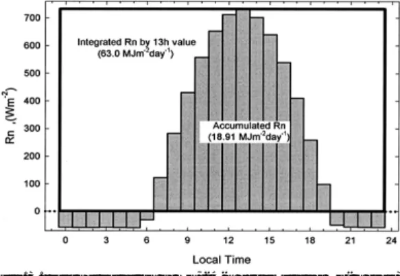
Fig. 3. shows the hourly mean value for study period and stations of Rn. The maximum value is presented at 13:000 LST. The integrated Rn value (thick rectangle in Fig. 3) by this maximum value is 63.0 MJm-2day-1, while the 24-h accumulated Rn value (part filled in gray) is 18.91 MJm-2day-1. Since it was previously assumed that the ratio of instantaneous net radiation Rniand of the 13:00LST net radiation Rnmequals 1, the following relationship can be established;
C = = (8)
where C is the radiation ratio, Rndis the daily net radiation flux (Wm-2), Rniis the instantaneous net radiation (Wm-2), and Rnmis the daily maximum (13:00 LST) net radiation (Wm-2), which allows estimating Bd from Bhor Bmand a known C.
Rnd
Rnm
Rnd
Rni
z0_g5
g3
LT_g4
g2
1 2
Table 2. Typical values of the plant height, the zero-plane displacement and the roughness length for the present land covers.
Land cover Plant height h,Roughness Length z0, Zero-plane (m) (m) displacement d, (m)
Needle leaf Forest 10.7 1.40 7.2
Broad leaf Forest 6.15 0.85 4.1
Shrub land 0.77 0.10 0.5
Crop land 0.46 0.06 0.3
Grass land 0.15 0.02 0.1
Barren land 0.08 0.01 0.05
Land cover Plant height h,Roughness Length z0, Zero-plane (m) (m) displacement d, (m)
Fig. 3. Diurnal variation of Rn, 24-h accumulated Rn(in gray), and integrated Rn by maximum hourly value(thick rectangle).
Fig. 2. Bd values and Relationship between (ET - Rn) and (Ts- Ta) for z0values of 6 land cover types.
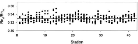
For summer, Seguin and Itier (1983) reported a mean C value of 0.3, but a standard deviation (0.03) that is to large too be neglected and consequently that preclude the simple usage of Eq. (8). The distribution of C values is depicted in Fig. 4 and the results from the present study revealed that C ranges from 0.316 to 0.353 for all cover classes, with a mean value of 0.331 and a much lower standard deviation (0.0073) that, we believe, could be neglected for daily apparent ET* estimations.
The Gaussian model proposed for Bh(Eq. (7)) could thus be easily adapted for Bd, implying only a unit adjustment from mm h-1K-1to mm d-1K-1.
Assuming that C equals 0.331 for all land covers and the validity of Eq. (8), Eq. (6) may be written as follow:
ETd= 0.331·[Rnm_c·(Tsm_Tam*)] (9) where c is a coefficient (mm·h-1K-1).
The value of c is shown in Fig. 5, along Bmcomputed through the proposed Gaussian model (Eq. (7)), as a function of z0. Both coefficients show a good agreement to one another, the largest difference occurring at z0
values 0.1 m and 1.4 m. Therefore, C could be approximated by
c= » Bm (10)
which implies that Bmcan substitute c in the Eq. (9).
The resumes of the input values that this study has applied for the two algorithms are as follows;
1) Method of Jackson et al.
- Tsmfrom the split window method of Ulivieri et al.
(1994) (Eq. (3))
- Use of Tamfrom meteorological station measurement.
- Bdobtained from relationship between terms (Tsm- Tam) and (ETd- Rnd).
- Rndcalculated by daily net radiation model.
- ETdcalculated by equation of Jackson et al. (1977) (Eq. (2)).
2) Present algorithm - Tsm(same algorithm above).
- Tam*the third-order polynomial multiple regression (Eq. (4)).
- Bmobtained by Gaussian model for estimation Bh (Eq. (7)).
- Rnmobtained by instantaneous net radiation model.
- ETdcalculated by Eq. (9) and (10).
A comparison of the apparent daily ET* from the original B-method of Jackson et al. (1977) and from the proposed extension of Bm(i.e. Bm×24) is given in Fig.
6. Both estimations agree to each other (R2 = 0.99 and the regression line slope is 0.99; SE and RMSE are 0.18 and 0.26 mm/day). Errors reach 0.5mm/day for apparent ET* larger than about 8mm/day, which is by no means a fatal inaccuracy.
7. Conclusions
The proposed daily apparent ET* system was compared to the original B method of Jackson et al.
Bd C
Fig. 4. Scatter plot for the distribution of net radiation ratio
Fig. 5. Coefficients C (circle) and Bm(triangle) as a function of z0.
(1977). Residuals of the proposed system were randomly distributed, but increased slightly with increasing the ET* values (maximum 0.5 mm/day). It is assumed that these errors were due to the difference in the Bmand c values. In particular, these differences for the z0= 0.1m (shrub land) and z0= 1.4m (needle-leaf forest) are thought. It may be argued that the presumption of Bmby hourly Gaussian model for B, which is strictly based on the surface roughness length and local time, does not depict perfectly the time distribution of the wind velocity influence. In spite of this approximation, the estimation scheme accurately represents daily evapotranspiration values obtained by the method of Jackson et al. (1977) (the fitted line y = 0.99x - 0.18; R2= 0.99) and the agreement is very encouraging because this may offer more rapid estimation and reduced data volume.
Acknowledgments. This study was supported by funds from SOPFEU. Satellite data were kindly provided by Environment Canada. Ground-based data were kindly provided by SOPFEU, Environment Canada, and the POMMIER network. Finally, the authors would like to thank for the useful comments of anonymous reviewers.
References
Bussieres, N. and P. Y. T. Louie, 1989. Implementation of an algorithm to estimate regional evapotranspiration using satellite data, Rapport de recherche Environ. Atmos. Canada, Downsview, 26p.
Carlson, T. N. and F. E. Boland, 1978. Analysis of urban-rural canopy using a surface heat flux/temperature model, J. Appl. Meteorol., 17:
998-1013.
Carlson, T. N. and M. J. Buffum, 1989. On estimating total daily evapotranspiration from remote surface temperature measurement, Remote Sens.
Environ., 29: 197-207.
Carlson, T. N., J. K. Dodd, S. G. Benjamin, and J. N.
Cooper, 1981. Satellite estimation of the surface energy balance, moisture availability and thermal inertia, J. Appl. Meteorol., 20: 67-87.
Coll, C., V. Caselles and T. J. Schmugge, 1994a.
Estimation of land surface emissivity differences in the split-window channels of AVHRR, Remote Sens. Environ., 48: 127-134.
Cooper, D. I. and G. M. Asrar, 1989. Evaluating atmospheric correction models for retrieving surface temperatures from the AVHRR over a tallgrass prairie, Remote Sens. Environ., 27: 93- 102.
Gurney, R. J. and D. K. Hall, 1983. Satellite-derived surface energy balance estimates in the Alaskan sub-arctic, J. Clim. Appl. Meteorol., 22: 115- 125.
Han, K. S., A. A. Viau, and F. Anctil, 2003 a. Hourly apparent evapotranspiration mapping based on GOES/IMAGER and NOAA/AVHRR data combination, ISPRS J. Photogram. Remote Sens., submitted.
Han, K. S., A. A. Viau, and F. Anctil, 2003 b. High Fig. 6. Scatter plot of the daily apparent ET* system results
and of the B-method results.
resolution forest Fire-Weather Index computations using satellite remote sensing.
Can. J. Forest Res., 33(6): 1134-1143.
Jackson, R. D., 1985. Evaluating evapotranspiration at local and regional scales, In the Proceeding IEEE, 73: 1086-1096.
Jackson, R. D., R. J. Reginato, and S. B. Idso, 1977.
Wheat canopy temperature: a practical tool for evaluating water requirements, Water Resour.
Res., 13(3): 651-656.
Monteith, J. L. and M. H. Unsworth, 1990. Principles of environmental physics, Edward Arnold, New York.
Moran, M. S. and R. D. Jackson, 1991. Assessing the spatial distribution of evapotranspiration remotely sensed inputs, J. Environ. Qual., 20:
725-737.
Price, J. C., 1980. The potential of remotely sensed thermal infrared data to infer surface soil moisture and evaporation, Water Resour. Res., 16: 787-795.
Price, J. C., 1982. Estimation of regional scale evapotranspiration through analysis of satellite thermal-infrared data, IEEE Trans. Geosci.
Remote Sens., 20: 286-292.
Running, S. W., R. R. Nemani, D. L. Peterson, L. E.
Band, D. F. Potts, L. L. Pierce, and M. A.
Spanner, 1989. Mapping regional forest evapotranspiration and photosynthesis by coupling satellite data with ecosystem
simulation, Ecology, 704: 1090-1101.
Seguin, B., and B. Itier, 1983. Using midday surface temperature to estimate daily evaporation from satellite thermal IR data, Int. J. Remote Sens., 4:
371-383.
Soer, G. J. R., 1980. Estimation of regional evapotranspiration and soil moisture conditions using remotely sensed crop surface temperatures, Remote Sens. Environ., 9: 27-45.
Stannard D. I., 1993. Comparison of Penman-Monteith, Shuttleworth- Wallace, and modified Priestley- Taylor Evapotranspiration models for wildland vegetation in semiarid rangeland, Water Resour.
Res., 29(5): 1379-1392.
Taconet, O., R. Bernard and D. Vidal-Madjar, 1986.
Evapotranspiration over an agricultural region using a surface flux/temperature model based on NOAA-AVHRR data, J. Clim. Appl. Meteorol., 25: 284-307.
Ulivieri, C., M. M. Castronouvo, R. Francioni, and A.
Cardillo, 1994. A split-window algorithm for estimating land surface temperature from satellites, Adv. Space Res., 14(3): 59-65.
Viau, A. A., J. V. Vogt, and F. Paquet, 1996.
Regionalisation and Mapping of Air Temperature Fields Using NOAA AVHRR Imagery, Actes du 9e Congres de l’Association quebecoise de teledetection (AQT): La teledetection au sein de la geomatique, Quebec, Canada, CD-ROM.