Numerical Simulation of Overtopping of Cnoidal Waves on a Porous Breakwater Using the Boussinesq Equations: Comparison with Solutions of the Navier-Stokes Equations

(1)

https://doi.org/10.9765/KSCOE.2019.31.2.41

41

Numerical Simulation of Overtopping of Cnoidal Waves on a Porous Breakwater Using the Boussinesq Equations: Comparison with Solutions

of the Navier-Stokes Equations

Boussinesq 식을 사용하여 Cnoid 파의 투수방파제 월파 해석:

Navier-Stokes 식 결과와 비교

Thanh Thu Huynh, Changhoon Lee and Suk Jin Ahn 휜탄트* · 이창훈* · 안석진**

Abstract : We approximately obtain heights of cnoidal waves overtopping on a porous breakwater using both the one-layer Boussinesq equations (Vu et al., 2018) and the two-layer Boussinesq equations (Huynh et al., 2017). For cnoidal waves overtopping on a porous breakwater, we find through numerical experiments that the heights of cnoidal waves overtopping on a low-crested breakwater (obtained by the Navier-Stokes equations) are smaller than the heights of waves passing through a high-crested breakwater (obtained by the one-layer Boussinesq equations) and larger than the heights of waves passing through a submerged breakwater (obtained by the two-layer Boussinesq equations). As the cnoidal wave nonlinearity becomes smaller or the porous breakwater width becomes narrower, the heights of transmitting waves obtained by the one-layer and two-layer Boussinesq equations become closer to the height of overtopping waves obtained by the Navier-Stokes equations.

Keywords : Boussinesq equations, Navier-Stokes equations, porous breakwater, overtopping, cnoidal waves, numerical experiment

요 지 :1개층 Boussinesq 방정식(Vu 등, 2018)과 2개층 Boussinesq 방정식(Huynh 등, 2017)을 사용하여 투수방파 제를 지나는 cnoid 파의 월파고를 구하였다. 수치실험을 통해 천단고가 낮은 투수방파제를 지나는 cnoid 파의 월 파고(Navier-Stokes 방정식으로 구함)가 천단고가 높은 투수방파제를 지나는 통과파고(1개층 Boussinesq 방정식으로 구함)보다 더 작고, 천단고가 해저에 있는 투수방파제를 지나는 통과파고(2개층 Boussinesq 방정식으로 구함)보다 더 크다는 것을 확인하였다. cnoid 파의 파고가 낮을수록 또는 투수방파제의 폭이 좁을수록 1개층 및 2개층 Boussinesq 방정식으로 구한 통과파고가 Navier-Stokes 방정식으로 구한 월파고에 근접한 것을 확인하였다.

핵심용어 :Boussinesq 방정식, Navier-Stokes 방정식, 투수 방파제, 월파, cnoid 파, 수치실험

1. Introduction

Wave overtopping on a breakwater may cause damage to coastal structures as well as injuries and the loss of life to people. In reality, wave overtopping is a three-dimensional phenomenon due to refraction and diffraction because usu- ally waves propagate obliquely on coastal structures. Usu- ally, people use three-dimensional equations such as the Reynolds Averaged Navier-Stokes equations, e.g., COBRAS (Lin and Liu, 1998) and CASMAS-SURF (CDIT, 2001) or the smooth particle hydrodynamics method (Gingold and

Monaghan, 1977) to simulate wave overtopping. Simula- tion of the three-dimensional equations in a horizontal two- dimensional domain requires so much storage and so long execution time. Hence, coastal engineers simulate wave overtopping mostly for normally incident waves. The Boussinesq equations are depth-averaged two-dimensional equations. Thus, simulation of the Boussinesq equations in a horizontal two-dimensional domain does not require so much storage nor such a long execution time. Cruz et al.

(1997) developed the Boussinesq equations for waves on a porous bed. The equations consider waves in two layers,

**세종대학교 건설환경공학과 (Corresponding author: Changhoon Lee, Department of Civil & Environmental Engineering, Sejong University, Seoul 05006, Korea, Tel: +82-2-3408-3294, Fax: +82-2-3408-4332, [email protected])

**(주)지오시스템리서치 부설연구소(Research Institute, GeoSystem Research Corporation)

(2)

i.e., an upper water layer and a lower porous layer. Recently, Huynh et al. (2017) extended Cruz et al.’s Boussinesq equations to analyze waves in two porous layers with different porosities. Also, Vu et al. (2018) developed the Boussinesq equations for waves in one porous layer. The waves overtopping on a low-crested porous breakwater would experi- ence energy dissipation more than waves through a high- crested breakwater and less than waves passing through a submerged porous breakwater. Thus, the heights of waves overtopping on a low-crested porous breakwater which can be simulated using the Navier-Stokes equations would be greater than those of waves passing through a high-crested porous breakwater which can be simulated using the one-

layer Boussinesq equations (Vu et al., 2018) and also those are less than those of waves passing through a submerged breakwater which can be simulated using the two-layer Boussinesq equations (Cruz et al., 1997). Fig. 1 shows three cases of cnoidal waves passing on a porous breakwater. Recently, Huynh et al. (2017) approximately simulated overtopping of solitary waves on a porous breakwater using the extended Boussinesq equations. The results of the Boussinesq equations are well compared with those of the CADMAS-SURF which uses the Navier-Stokes equations (CDIT, 2001). Solitary waves are long waves, have infinitely large wavelength and are used to represent earthquake-induced tsunamis. Another type of long waves are cnoidal waves which have finite wavelength and are used to represent wind waves. In Korea, wind waves are more common than tsunamis.

In this study, we approximately simulate overtopping of cnoidal waves on a porous breakwater. The numerical results are compared to the results of the Navier-Stokes equation model CADMAS-SURF. In Section 2, we describe governing equations of the one-layer and two-layer Bouss- inesq equations and the Navier-Stokes equations and also drag and inertial resistances. In Section 3, we conduct numerical experiments to find optimum values of the drag and inertial resistance coefficients which are used in the Boussinesq equations and the Navier-Stokes equations and to find the heights of cnoidal waves overtopping on a low- crested porous breakwater are between those of cnoidal waves passing through a high-crested porous breakwater and a submerged porous breakwater. In section 4, we sum- marize the present study and suggest the future study.

2. Governing Equations with Resistances

2.1 Drag and Inertial Resistances

Wave energy dissipation in porous media occurs domi- nantly via the turbulence of high speed waters and also by the friction of waters through porous media. These are called the turbulent and laminar drag resistances, respectively. The energy dissipation also occurs due to unsteadiness of water waves in porous media so-called inertial resistance. The momentum equation in porous media can be given as

(1)

where λ is the porosity, U = (u, v, w) is the seepage velocity vector, p is the pore pressure, ρ is water density, g is the gravitational acceleration, D is the drag resistance

λ dU --- + dt 1

ρ --- ∇

3

( p + ρgz ) + D + I = 0

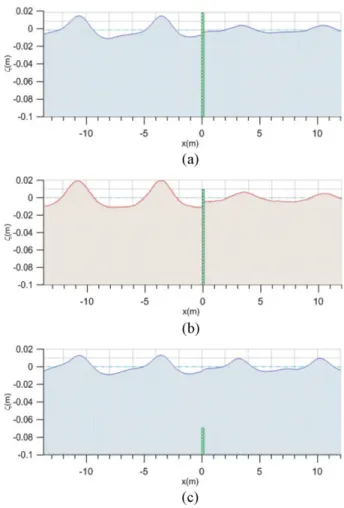
Fig. 1. Conceptual surface elevations of cnoidal waves overtopping on a porous breakwater: (a) high-crested breakwater, (b) low-crested breakwater, (c) submerged breakwater.

(3)

term, and I is the inertial resistance term, and ∇

₃

≡(∂/∂x, ∂/

∂y, ∂/∂z) is the gradient operator. There are several ways to define the drag resistance term. Ergun (1952) defined the drag resistance term using a volume-averaged discharge velocity U'(= λU). In the presents study, we use Ergun’s definition of D in terms of the seepage velocity U instead:

(2)

where α

l

and α

t

are coefficients representing the laminar and turbulent flow resistances, respectively, ν is the kine- matic viscosity of water, and d is the size of the solid material. Engelund (1953) also used the Forchheimer type to define the drag resistance term:

(3)

where α

lE

and α

tE

are coefficients which represent the laminar and turbulent flow resistances, respectively, recom- mended by Engelund. The inertial resistance term I in Eq.

(1) is given by

(4)

where κ is the added mass coefficient.

Substitution of Eqs. (2) and (4) into the momentum equation (1) gives

(5)

where the inertial resistance coefficient β is

(6) and the drag resistance coefficient α is

(7)

We use the CADMAS-SURF (CDIT, 2001) for the Navier-Stokes equations model. The CADMAS-SURF was developed by the Coastal Development Institute of Tech- nology, Japan. In the CADMAS-SURF, the momentum equation can be expressed as

(8)

where β

c

= λ + (1 − λ)(1 + κ) and α = α

lE

[(1 − λ)

³

/λ

²

]ν/d

²

+ α

tE

[(1 − λ)/λ]|U|/d are the inertial and drag resistance coefficients (Engelund, 1953), respectively, α

lE

and α

tE

are the laminar and turbulent drag resistance coefficients, respectively, suggested by Engelund. The inertial and drag resistance coefficients between eqs. (5) and (8) are related as

β = β

c

, α

l

= λ(1 − λ)α

lE

, α

t

= α

tE

(9)

2.2 Governing Equations

The extended Boussinesq equations for waves in one porous layer derived by Vu et al. (2018) are given by

(10)

(11)

where u(= (u, v)) is the depth-averaged horizontal seepage velocity vector, γ(= 1/18) is a parameter to improve the dispersion relation in deeper water. For the water layer (i.e., β = 1 and α = 0), the momentum equation (11) becomes Madsen and Sørensen’s (1992) equation given by

(12)

The extended Boussinesq equations for waves in two porous layers derived by Huynh et al. (2017) are given by

(13)

(14) D = α

l

1 − λ

--- λ

⎝ ⎠

⎛ ⎞ ν

d

²

---U '

--- + α λ

t

1 − λ --- λ 1

d --- U ' --- U λ '

--- λ

D = αl

1 − λ

--- λ

⎝ ⎠

⎛ ⎞ ν

d

²

--- U + α

t

1 − λ --- λ 1

d --- U U

D = α

lE

( 1 − λ )

³

--- ν λ

d

²

---U '

--- + α λ

tE

1 − λ --- λ 1

d --- U ' --- U λ '

--- λ

I = 1 ( − λ ) 1 + κ ( ) d U --- dt

β d U --- + dt 1

ρ --- ∇

₃

( p + ρgz ) + αU = 0

β = λ + 1 − λ ( ) 1 + κ ( )

α = α

l

1 − λ --- λ

⎝ ⎠

⎛ ⎞ ν

d

²

--- + α

t

1 − λ --- λ 1

d --- U

β

c

dU --- + λ dt

ρ --- ∇

₃

( p + ρgz ) + α

c

U = 0

∂ζ

--- + ∇ ∂t ⋅ [ ( h + ζ )u ] = 0

β ∂ ∂t ---- + α

⎝ ⎠

⎛ ⎞u + βu ∇u + g∇ζ + 1 ⋅ 6 --- ⎝ ⎛ β ∂ ∂t ---- + α ⎠ ⎞h

²

∇ ∇ u ( ⋅ )

− 1 2 --- + γ

⎝ ⎠

⎛ ⎞ β ∂ ⎝ ⎛ ∂t ---- + α ⎠ ⎞h∇ ∇ hu [ ⋅ ( ) ]

− γgh∇ ∇ h∇ζ [ ⋅ ( ) ] = 0

∂u ∂t

--- + u ∇u + g∇ζ + 1

6 ---h

²

∇ ∇ ∂u ⎝ ⎛ ⋅ --- ∂t ⎠ ⎞

⋅

− 1 2 --- + γ

⎝ ⎠

⎛ ⎞h∇ ∇ h∂u --- ∂t

⎝ ⎠

⎛ ⎞

⋅ − γgh∇ ∇ h∇ζ [ ⋅ ( ) ] = 0

∂ζ

--- + ∇ ∂t [ ( h

₁

+ ζ )u

₁

] + λ

₂

λ

₁

--- ∇ [ ( h

₂

− h

₁

)u

₂

] = 0

⋅ ⋅

β

₁

∂

∂t ---- + α

₁

⎝ ⎠

⎛ ⎞u

1

+ β

₁

u

₁

∇u

₁

+ g∇ζ + 1 2 --- β

₁

∂

∂t ---- + α

₁

⎝ ⎠

⎛ ⎞

⋅ h

₁²

--- 3 ∇ ∇ u ( ⋅

₁

) − h

₁

∇ λ

₂

λ

₁

--- ∇ ⋅ [ ( h

₂

− h

₁

)u

₂

]

⎩ ⎭

⎨ ⎬

⎧ ⎫

− 1 2 --- + γ

₁

⎝ ⎠

⎛ ⎞ β

1

∂

∂t ---- + α

₁

⎝ ⎠

⎛ ⎞h

₁

∇ ∇ h [ ⋅ (

₁

u

₁

) ]

− γ

₁

gh

₁

∇ ∇ h [ ⋅ (

₁

∇ζ ) ] = 0

β

₂

∂

∂t ---- + α

₂

⎝ ⎠

⎛ ⎞u

2

+ β

₂

u

₂

⋅ ∇u

₂

+ g∇ζ + 1 2 --- β

₂

∂

∂t ---- + α

₂

⎝ ⎠

⎛ ⎞

− 2

3 --- h (

₂

− h

₁

)

²

∇ ∇ u ( ⋅

₂

) − h (

₂

− h

₁

)∇ ∇h (

₂

⋅ u

₂

)

(4)

(15)

where γ

₁

(= 1/18), γ

₂

(= 1/18) are parameters to improve the dispersion relation in deeper waters, the subscripts 1 and 2 imply the associated variables are in the upper and lower layers, respectively. If β

₁

= 1, α

₁

= 0, λ

₁

= 1, that is, the upper layer is filled with water, then Eqs. (13) to (15) become Cruz et al.’s (1997) Boussinesq equations. Cruz et al.’s equations can be applied for waves on porous beds and submerged breakwaters. The present equations can be applied further for waves in two porous layers with different porosities.

The continuity and momentum equations of the CAD- MAS-SURF (CDIT, 2001) can be expressed as

(16)

(17)

where S

_ρ

and S

_u

are source terms in the continuity and momentum equations, respectively. At the free surface, the transport equation of F is used as

(18)

where F is the volume of fluid and S

_F

is the source term of F.

3. Numerical Experiments

3.1 Numerical Schemes

We use the finite-difference method to solve the extended Boussinesq equations (10) and (11) for one porous layer and the equations (13)~(15) for two porous layers. The time derivative terms are discretized with the Adam-Bashforth- Moulton predictor and corrector scheme following the FUNWAVE (Kirby et al., 1998). In the present study, we simulate wave propagation in horizontally one-dimensional case.

For waves in one porous layer, Eqs. (10) and (11) can be rewritten as

(19) (20) where

(21)

(22)

(23)

The subscripts in Eqs. (19)~(23) imply that the term is taken derivative with respect to the subscript. First, to discretize Eqs. (19) and (20) in time, we use the third-order Adams-Bashforth predictor scheme given by

(24)

(25)

where the superscripts n and n + 1 denote the present and the next time steps, respectively. The variable u

ⁿ⁺¹

which is included in U

ⁿ⁺¹

is calculated using the LU decomposition method. Second, to discretize Eqs. (19) and (20) in time, we use the fourth-order Adams-Moulton corrector scheme given by

(26)

(27)

For waves in two porous layers, Eqs. (13)~(15) can be rewritten as

(28) (29) (30) where

(31)

(32)

---

− h (

₂

− h

₁

)∇ h (

₂

− 2h

₁

)∇ u ⋅

₂

+ 2∇h

₂

∇h

₁

⋅ u

₂

− 1 2 --- β

₁

∂

∂t ---- + α

₁

⎝ ⎠

⎛ ⎞∇ ∇ h [ ⋅ (

12

u

₁

) ] − 1 + γ (

₂

) β

₁

∂

∂t ---- + α

₁

⎝ ⎠

⎛ ⎞

+ γ

₂

α

₂

β

₁

β

₂

--- − α

₁

⎝ ⎠

⎛ ⎞ ∇ h

1

λ

₂

λ

₁

--- ∇ ⋅ [ ( h

₂

− h

₁

)u

₂

]

⎩ ⎭

⎨ ⎬

⎧ ⎫

− γ

₂

g β

₁

β

₂

--- ∇ h

₁

λ

₂

λ

₁

--- ∇ ⋅ [ ( h

₂

− h

₁

)∇ζ ]

⎩ ⎭

⎨ ⎬

⎧ ⎫

= 0

∇

₃

⋅ ( ) = λS λu

_ρ

β

c

dU --- + λ dt

ρ --- ∇

₃

( p + ρgz ) + α

c

U = S

_u

λ∂ F

--- + ∇ ∂t

₃

⋅ ( λUF ) = λS

F

ζ

t

= E

₁

( ζ, u ) U u ( )

[ ]

_t

= F ( ζ, u )

E

₁

( ζ, u ) = − h + ζ [ ( )u ]

_x

U u ( ) = u + 1

6 ---h

²

u

_xx

− 1 2 --- + γ

⎝ ⎠

⎛ ⎞h hu ( )

xx

F ( ζ, u ) = − α β ---u − g

β --- ζ

x

− uu

x

− 1 6 ---α

β ---h

²

u

_xx

+ 1

2 --- + γ

⎝ ⎠

⎛ ⎞α

---h hu β ( )

xx

+ γ

β ---gh hζ (

x

)

_xx

ζ

ⁿ⁺¹

= ζ

ⁿ

+ Δ t

12 --- 23E

₁ⁿ

− 16E

1n−1

+ 5E

₁ⁿ⁻²

( )

U

ⁿ⁺¹

= U

ⁿ

+ Δ t

12 --- 23F (

ⁿ

− 16F

ⁿ⁻¹

+ 5F

ⁿ⁻²

)

ζ

ⁿ⁺¹

= ζ

ⁿ

+ Δ t

24 --- 9E (

₁ⁿ⁺¹

+ 19E

₁ⁿ

− 5E

₁ⁿ⁻¹

+ E

₁ⁿ⁻²

)

U

ⁿ⁺¹

= U

ⁿ

+ Δ t

24 --- 9F (

ⁿ⁺¹

+ 19F

ⁿ

− 5F

ⁿ⁻¹

+ F

ⁿ⁻²

)

ζ

t

= E

₂

( ζ, u

₁

, u

₂

) U

₁

( ) u

₁

[ ]

_t

= F

₁

( ζ, u

₁

, u

₂

) + H [

₁

( ) u

₂

]

_t

U

₂

( ) u

₂

[ ]

_t

= F

₂

( ζ, u

₁

, u

₂

) + H [

₂

( ) u

₁

]

_t

E

₂

( ζ, u

₁

, u

₂

) = − h [ (

₁

+ ζ )u

₁

]

_x

− λ

₂

λ

₁

--- h [ (

₂

− h

₁

)u

₂

]

_x

U

₁

( ) = u u

₁ ₁

+ 1

6 ---h

₁²

u

_1xx

− 1 2 --- + γ

₁

⎝ ⎠

⎛ ⎞h

₁

( h

₁

u

₁

)

_xx

(5)

(33)

(34)

(35)

(36)

(37)

First, to discretize Eqs. (28)~(30) in time, we use the third-order Adams-Bashforth predictor scheme given by

(38)

(39)

(40)

The variables u

₁ⁿ⁺¹

and u

₂ⁿ⁺²

which are included in both U

₁ⁿ⁺¹

(u

₁

, u

₂

) and U

₂ⁿ⁺¹

(u

₁

, u

₂

) are calculated using the LU decomposition method. Second, to discretize Eqs. (28) - (30) in time, we use the fourth-order Adams-Moulton corrector scheme given by

(41)

(42)

(43)

3.2 Determination of Optimal Values of Drag and Inertial Resistance Coefficients

To simulate wave propagation and energy dissipation in porous media, we need to determine values of inertial and drag resistance coefficients. In the inertial resistance coefficient β given by Eq. (6), we use the value of added mass coefficient as κ = 0.34 which was suggested by Lara et al.

(2012) for waves in a porous breakwater. In simulating the Boussinesq equations, Vu et al. (2018) found optimal values of the laminar and turbulent drag resistance coefficients α

l

= 800 and α

t

= 3 which give minimum root-mean- squared relative errors between the transmission coefficients by the Boussinesq equations and those of Vidal et al.’s (1988) hydraulic experimental data. In simulating the Boussinesq equations for waves in one and two porous layers, we use Vu et al.’s suggested values of the laminar and turbulent drag resistance coefficients.

In the present study, to simulate the CADMAS-SURF for waves in one and two porous layers, we find optimal values of the laminar and turbulent drag resistance coefficients α

lE

and α

tE

following Vu et al.'s approach. Vidal et al.

conducted hydraulic experiments to measure transmission coefficients of solitary waves passing through a porous breakwater. The experimental conditions of Vidal et al. are given in Table 1. We calculate the root mean squared relative error E

_r

of the transmission coefficients given by

(44)

where K

_tCAD

and K

_{t exp}

are the transmission coefficients obtained by the CADMAS-SURF and the Vidal et al.’s F

₁

( ζ, u

₁

, u

₂

) = − α

1

β

₁

---u

₁

− u

₁

u

_1x

− g β

₁

--- ζ

_x

− 1

6 --- α

1

β

₁

---h

₁²

u

_1xx

+ 1 2 --- + γ

₁

⎝ ⎠

⎛ ⎞α

¹

β

₁

---h

₁

( h

₁

u

₁

)

_xx

+ γ

₁

β

₁

---gh

₁

( h

₁

ζ

x

)

_xx

+ 1 2 --- α

₁

β

₁

--- λ

₂

λ

₁

---h

₁

[ ( h

₂

− h

₁

)u

₂

]

_xx

H

₁

( ) = u

₂

1 2 ---h

₁

λ

₂

λ

₁

--- h [ (

₂

− h

₁

)u

₂

]

_xx

U

₂

( ) = u u

₂ ₂

− 1

3 --- h (

₂

− h

₁

)

²

u

_2xx

− 1

2 --- h (

₂

− h

₁

) h (

_2x

u

₂

)

_x

− 1

2 --- h (

₂

− h

₁

) h (

₂

− 2h

₁

)

x

u

_2x

+ h

_1x

h

_2x

u

₂

− 1 + γ (

₂

) β

₁

β

₂

--- λ

₂

λ

₁

--- h {

₁

[ ( h

₂

− h

₁

)u

₂

]

_x

}

_x

F

₂

( ζ, u

₁

, u

₂

) = − α

₂

β

₂

---u

₂

− u

₂

u

_2x

− g β

₂

--- ζ

x

+ 1 3 --- α

2

β

2

--- h (

₂

− h

₁

)

²

u

_2xx

+ 1 2 --- α

2

β

2

--- h (

₂

− h

₁

) h (

_2x

u

₂

)

_x

+ 1 2 --- α

₂

β

₂

--- h (

₂

− h

1

) h (

2

− 2h

1

)

x

u

_2x

− α

₂

β

₂

---h

_1x

h

_2x

u

₂

− α

₁

β

₂

--- + γ

₂

α

₂

β

₁

β

₂²

---

⎝ ⎠

⎛ ⎞λ

²

λ

₁

--- h {

₁

[ ( h

₂

− h

₁

)u

₂

]

_x

}

_x

+ γ

₂

g β

1

β

2

--- λ

2

λ

1

--- h {

₁

[ ( h

₂

− h

₁

)ζ

x

]

_x

}

_x

+ 1 2 --- α

1

β

2

--- h (

₁²

u

₁

)

xx

H

₂

( ) = u

₁

1 2 --- β

₁

β

2

--- h (

₁²

u

₁

)

xx

ζ

ⁿ⁺¹

= ζ

ⁿ

+ Δ t

12 --- 23E (

₂ⁿ

− 16E

₂ⁿ⁻¹

+ 5E

₂ⁿ⁻²

)

U

₁ⁿ⁺¹

= U

₁ⁿ

+ Δ t

12 --- 23F (

₁ⁿ

− 16F

₁ⁿ⁻¹

+ 5F

₁ⁿ⁻²

) + 2H

₁ⁿ

− 3H

₁ⁿ⁻¹

+ H

₁ⁿ⁻²

U

₂ⁿ⁺¹

= U

₂ⁿ

+ Δ t

12 --- 23F (

₂ⁿ

− 16F

₂ⁿ⁻¹

+ 5F

₂ⁿ⁻²

) + 2H

₂ⁿ

− 3H

2n−1

+ H

₂ⁿ⁻²

ζ

ⁿ⁺¹

= ζ

ⁿ

+ Δ t

24 --- 9E (

₁ⁿ⁺¹

+ 19E

₁ⁿ

− 5E

₁ⁿ⁻¹

+ E

₁ⁿ⁻²

)

U

₁ⁿ⁺¹

= U

₁ⁿ

+ Δ t

24 --- 9F (

₁ⁿ⁺¹

+ 19F

₁ⁿ

− 5F

₁ⁿ⁻¹

+ F

₁ⁿ⁻²

) + H

₁ⁿ⁺¹

− H

₁ⁿ

U

₂ⁿ⁺¹

= U

₂ⁿ

+ Δ t

24 --- 9F

₂ⁿ⁺¹

+ 19F

₂ⁿ

− 5F

2n−1

+ F

₂ⁿ⁻²

( )

+ H

₂ⁿ⁺¹

− H

₂ⁿ

E

_r

= 1

N ---- K

_{tCAD n}

− K

_{t exp n}

K

_{t exp n}

---

⎝ ⎠

⎜ ⎟

⎛ ⎞

²

n=1

∑

N

Table 1. Experimental conditions of Vidal et al. (1988) for solitary waves in a porous breakwater

Case h (m) b (m) d (m) λ

1 0.300 0.2 0.0143 0.44

2 0.300 0.4 0.0134 0.44

3 0.302 0.2 0.0243 0.44

4 0.317 0.4 0.0243 0.44

5 0.301 0.2 0.0315 0.42

6 0.301 0.4 0.0315 0.42

(6)

data, respectively, and N is the total number of the transmission coefficients in each case. We compare averaged values of E

_r

for the 6 total cases and then choose optimal values of α

lE

and α

tE

which yield the smallest averaged error. Table 2 shows the root mean squared relative errors with the different drag resistance coefficients of α

lE

= 1000, 2000, 3000 and α

tE

= 0, 1, 2. Finally, the drag resistance coefficients of α

lE

= 2000 and α

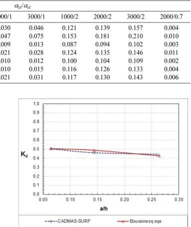
tE

= 0.7 are found to yield the smallest averaged error.

Fig. 2 shows the variation of transmission coefficients with wave nonlinearity for models with α

l

= 800, α

t

= 3 (Boussinesq equations), and α

lE

= 2000 and α

tE

= 0.7 (CADMAS-SURF). The CADMAS-SURF with α

lE

= 2000 and α

tE

= 0.7 as well as the Boussinesq equations with α

l

= 800, α

t

= 3 yields close solutions to the hydraulic experimental data. Hence, optimal values of the drag resistance coefficients are determined as α

lE

= 2000 and α

tE

= 0.7 in the CADMAS-SURF.

We also investigate the energy dissipation coefficient for waves in a porous breakwater. The energy dissipation coefficient can be defined as

(45) Fig. 3 shows the variation of energy dissipation coefficients with wave nonlinearity with the optimum values of the drag resistance coefficients. It is noticeable that, even without experimental data, numerical solutions of the energy dissipation coefficient are close to each other between the Boussinesq equations and the CADMAS-SURF. It is inter- esting that the energy dissipation coefficient decreases slightly with the increase of wave nonlinearity. Figs. 2 and 3 show that, as wave nonlinearity increases, the increase of the reflection coefficient is more significant than the decrease of the transmission coefficient and thus the energy dissipation coefficient would decrease.

3.3 Numerical Simulation of Overtopping of Cnoidal Waves on a Porous Breakwater

The surface elevation of cnoidal waves can be expressed as

(46) K

_d

= 1 − K

R

2

− K

T 2

ζ

^I

= ζ

tr

+ H Cn

²

2K

₁

t T ---|m

⎝ ⎠

⎛ ⎞

Table 2. Root mean squared relative errors of transmission coefficients of the CADMAS-SURF model against those of Vidal et al.’s experiment

Case αlE/αtE

1000/0 2000/0 3000/0 1000/1 2000/1 3000/1 1000/2 2000/2 3000/2 2000/0.7

1 1.392 0.737 0.393 0.017 0.030 0.046 0.121 0.139 0.157 0.004

2 2.962 1.242 0.514 0.025 0.047 0.075 0.153 0.181 0.210 0.010

3 1.247 0.976 0.765 0.005 0.009 0.013 0.087 0.094 0.102 0.003

4 3.165 2.292 1.649 0.016 0.021 0.028 0.124 0.135 0.146 0.011

5 1.366 1.157 0.983 0.007 0.010 0.012 0.100 0.104 0.109 0.002

6 3.041 2.418 1.904 0.006 0.010 0.015 0.116 0.126 0.133 0.004

Aver. 2.196 1.470 1.035 0.013 0.021 0.031 0.117 0.130 0.143 0.006

Fig. 2. Variation of transmission coefficients with nonlinearity for models with αl= 800, αt= 3 (Boussinesq equations) and αlE= 2000 and αtE= 0.7 (CADMAS-SURF).

Fig. 3. Variation of energy dissipation coefficients with wave nonlinearity for models with αl= 800, αt= 3 (Boussinesq equations) and αlE= 2000 and αtE= 0.7 (CADMAS-SURF).

(7)

0.067, 0.133 and breakwater width of b = 5 cm, 10 cm, 20 cm, 30 cm.

Fig. 4 shows simulated water surface elevations at t = 7 sec for the high-crested breakwater (h

_c

= 60 cm), the low- crested breakwater (h

_c

= 1 cm), and the submerged breakwater (h

_c

= −7 cm) using the one-layer Boussinesq equations, the CADMAS-SURF, and the two-layer Boussinesq equations, respectively. The wave nonlinearity is a/h = 0.033 and the breakwater width is b = 5 cm. Wave overtopping and reflection have already happened at t = 7 s. High reflection and low transmission are seen for waves on the high-crested breakwater while low reflection and high transmission are seen for waves on the submerged breakwater.

Fig. 5 compares the transmission coefficients of cnoidal waves with different nonlinearities among the one- and two-layer Boussinesq equations and the CADMAS-SURF.

The transmission coefficients of waves overtopping a low- crested breakwater (obtained by the CADMAS-SURF) are greater than those of waves passing through a high-crested breakwater (obtained by the one layer Boussinesq equations) and less than those of waves passing through a submerged breakwater (obtained by the two layer Boussinesq equations). For waves with lower wave nonlinearity, overtopping waves can be predicted using the one-layer more accurately than two-layer Boussinesq equations.

Fig. 6 compares the reflection coefficients of cnoidal waves among the one-layer and two-layer Boussinesq equations and the CADMAS-SURF. The reflection coefficients of waves overtopping a low-crested breakwater are less than those of waves passing through a high-crested breakwater and greater than those of waves passing through a submerged breakwater.

(47)

where ζ

tr

is the elevation of wave trough, H is the height of incident waves, Cn is the Jacobian elliptic function, K

₁

and K

₂

are the complete elliptic integrals of the first and second kind, respectively, and m is the modulus to determine the wave shape.

For cnoidal wave overtopping, we get approximate solutions of the one-layer and two-layer Boussinesq equations and compare these with more accurate solutions of the CADMAS-SURF. Experimental conditions are water depth of h = 30 cm, breakwater width of b = 20 cm, porous material size of d = 1.43 cm, porosity of λ = 0.44. We simulate the wave heights passing through the breakwater for cnoidal waves in three cases such as high-crested breakwater with h

_c

= 60 cm, low-crested breakwater with h

_c

= 1 cm, and submerged breakwater with h

_c

= −7 cm (see Fig. 1). We get approximate solutions of wave overtopping for cnoidal waves with different conditions of nonlinearity a/h = 0.033,

ζ

tr

= H

m ---- 1 − m − K

₂

K

₁

---

⎝ ⎠

⎛ ⎞

Fig. 4. Surface elevations of cnoidal waves overtopping on a porous breakwater at t = 7 s (a/h = 0.033, b = 5 cm): (a) high-crested breakwater, (b) low-crested breakwater, (c) submerged breakwater.

Fig. 5. Variation of transmission coefficient with nonlinearity for cnoidal waves.

(8)

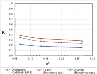
Fig. 7 compares the energy dissipation coefficients of cnoidal waves among the one-layer and two-layer Boussinesq equations and the CADMAS-SURF. The energy dissipation coefficients increase with the increase of wave nonlinearity.

The energy dissipation coefficients from the CADMAS- SURF are close to the one-layer Boussinesq equations. How- ever, the energy dissipation coefficients by the two layer Boussinesq equations are smaller than those by the one-layer Boussinesq equations and the CADMAS-SURF.

We also compare approximate solutions of cnoidal wave overtopping with different breakwater widths (b = 5 cm, 10 cm, 20 cm and 30 cm). For this numerical experiment, we keep initial conditions as the same as Vidal et al.’s experiment with nonlinearity a/h = 0.064. Fig. 8 shows that the transmission coefficients of waves overtoppinga low-crested breakwater (obtained by the CADMAS-SURF) are greater than those of waves passing through a high-crested break-

water (obtained by the one layer Boussinesq equations) and less than those of waves passing through a submerged

Fig. 6. Variation of reflection coefficient with nonlinearity for cnoi-

dal waves.

Fig. 10. Variation of energy dissipation coefficient with breakwater width for cnoidal waves.

Fig. 7. Variation of energy dissipation coefficient with nonlinearity for cnoidal waves.

Fig. 8. Variation of transmission coefficient with breakwater width for cnoidal waves.

Fig. 9. Variation of reflection coefficient with breakwater width for cnoidal waves.

(9)

breakwater (obtained by the two layer Boussinesq equations). Fig. 9 shows that the reflection coefficients of waves overtopping are slightly less than those of waves passing through a high-crest breakwater and higher than those of waves passing through a submerged breakwater.

Fig. 10 compares the energy dissipation coefficients among the one-layer and two-layer Boussinesq equations and the CADMAS-SURF. As the breakwater width becomes narrower, the energy dissipation would be negligibly smaller and thus the transmission and reflection coefficients would be near to unity and zero, respectively.

4. Conclusion

In the present study, we approximately obtain height of cnoidal waves overtopping on a porous breakwater using both the one-layer Boussinesq equations (Vu et al., 2018) and the two-layer Boussinesq equations (Huynh et al., 2017). For verification of the Boussinesq equations, we use the Navier-Stokes equations model CADMAS-SURF (CDIT, 2001). We use the value of added mass coefficient as κ = 0.34 which was suggested by Lara et al. (2012) for a porous breakwater. We use the drag resistances of Ergun (1952) and Engelund (1953) for the Boussinesq equations and the CADMAS-SURF, respectively. The values of laminar and turbulent drag resistances are determined such that the transmission coefficients of the models are close to those of Vidal et al.’s (1988) hydraulic experiment for solitary waves through a porous breakwater (i.e., one layer case).

Further, we find that the height of cnoidal waves overtopping on a low-crested breakwater (obtained by the Navier- Stokes equations) are smaller than the height of waves passing through a high-crested breakwater (obtained by the one- layer Boussinesq equations) and larger than the height of cnoidal waves passing through a submerged breakwater (obtained by the two-layer Boussinesq equations). As wave nonlinearity becomes smaller or the porous breakwater width becomes narrower, the heights of transmitting waves obtained by the one-layer and two-layer Boussinesq equations become closer to the height of overtopping waves obtained by the Navier-Stokes equations. If the water surface elevation is above the breakwater crest, the waves are in two layers, i.e., upper water layer and lower porous layer. If the water surface elevation is below the breakwater crest, the waves are in one porous layer. The present results for cnoidal waves are qualitatively the same as those for solitary waves (Huynh et al., 2017). In the future, we will directly simu-

late overtopping waves using both one-layer and two-layer Boussinesq equations simultaneously.

Acknowledgments

This research was supported by the Ministry of Science and ICT (No. 1711078047, title: Development of Predic- tion System for Marine Construction Schedule).

References

CDIT (2001). Research and development of a numerical wave flume;

CADMAS-SURF Report of the research group for development of numerical wave flume for the design of maritime structures.

Coastal Development Institute of Technology, Japan.

Cruz, E.C., Isobe, M. and Watanabe, A. (1997). Boussinesq equations for wave transformation on porous beds. Coastal Engi- neering, 30, 125-156.

Engelund, F.A. (1953). On the laminar and turbulent flows of ground water through homogeneous sand. Danish Academy of Technical Sciences.

Ergun, S. (1952). Fluid flow through packed columns. Chemical Engineering Progress, 48, 89-94.

Gingold, R.A. and Monaghan, J.J. (1977). Smoothed particle hydrodynamics: Theory and application to nonspherical stars.

Mon. Not. R. Astron. Soc., 181, 375-389.

Huynh, T.T., Lee, C. and Ahn, S.J. (2017). Numerical simulation of wave overtopping on a porous breakwater using Boussinesq equations. Journal of Korean Society of Coastal and Ocean Engineers, 29(6), 326-334.

Kirby, J.T., Wei, G., Chen, Q., Kennedy, A.B. and Dalrymple, R.A.

(1998). FUNWAVE 1.0 Fully nonlinear Boussinesq wave model documentation and user’s manual. Research report No. CACR- 98-06.

Lara, J.L., del Jesus, M. and Losada, I.J. (2012). Three-dimensional interaction of waves and porous coastal structures. Part II:

Experimental validation. Coastal Engineering, 64, 26-46.

Lin, P. and Liu, P.L.-F. (1998). A numerical study of breaking waves in the surf zone. Journal of Fluid Mechanics, 359, 239-264.

Madsen, P.A. and Sørensen, O.R. (1992). A new form of the Bouss- inesq equations with improved linear dispersion characteristics. Part 2: A slowly varying bathymetry. Coastal Engineering, 18, 183-204.

Vidal, C., Losada, M.A., Medina, R. and Rubio, J. (1988). Solitary wave transmission through porous breakwaters. Proc. 21st Inter- national Conference on Coastal Engineering, ASCE, 1073-1083.

Vu, V.N., Lee, C. and Jung, T.-H. (2018). Extended Boussinesq equations for waves in porous media. Coastal Engineering, 139, 85-97.

Received 3 March, 2019 Revised 26 March, 2019 Accepted 29 March, 2019