DOI : http://dx.doi.org/10.5394/KINPR.2013.37.3.283
Numerical Analysis of Waves coming with Oblique Angle to Submerged Breakwater on the Porous Seabed
†Nam-Hyeong Kim․Su-Min Woo*
†* Department of Civil Engineering/Marine & Environmental Research Institute, Jeju National University, Jeju 690-756, Republic of Korea
Abstract : Wave profiles coming with oblique angle to trapezoidal submerged breakwater on the porous seabed are computed numerically by using a boundary element method. The analysis method is based on the wave pressure function with the continuity in the analytical region including fluid and structure. When compared with the existing results on the oblique incident wave, the results of this study show good agreement. The fluctuation of wave profiles is increased in the rear of the submerged breakwater due to the increase of the transmission coefficient, as the incident angle increases. In addition, in the case of the wave profiles passing over the submerged breakwater on porous seabed, it is able to verify that the attenuation of wave height occurs more significantly due to the wave energy dissipation than that of passing over the submerged breakwater on the impermeable seabed. The results indicate that wave profile own high dependability regarding the change of oblique incident waves and porous seabed. Therefore, the results of this study are estimated to be applied as an accurate numerical analysis referring to oblique incident waves and porous seabed in real sea environment.
Key words :Boundary Element Method, Submerged Breakwater, Wave Pressure Function, Oblique Incident Waves, Porous seabed.
†Corresponding author, [email protected] 064) 754-3452
* [email protected] 064) 754-3453
1. Introduction
The development and utilization of ocean have been increasing as the economic and living condition have grown.
Also, before assessing the construction of structure in protecting a harbor and beach from ocean waves, the ability of an ocean engineer to predict wave profile passing on the porous seabed plays an important role. Wave dissipating structures such as the existing breakwater are showed over the surface of sea water. It is negative in terms of landscape and marine environment to block the flow of seawater. On the other hand, the submerged breakwater has several advantages in terms of the conservation of water quality and the landscape.
Ijima & Sasaki(1971) studied the effect of a submerged breakwater calculated using Domain Decompostion Method.
Chen et al.(2002) analyzed a thin submerged breakwater.
Their solution was based on the dual integral formulation for the modified Helmholtz equation. Takikawa &
Kim(1992), Kim(1995) and Kim & Woo(2012) analyzed the problem of the submerged breakwater in the case of impermeable seabed using the Wave Pressure Function.
In addition, Liu and Dalrymple(1984) obtained the solution
of laminar boundary layer on the porous seabed by replacing Darcy's law with the modified Dagan's porous flow model.
Kim et al.(2006) carried out the wave damping analysis in a porous seabed without oblique incident waves.
In this study the oblique incident waves are considered, and the objective of this paper is to analyze the wave profile passing over the trapezoidal submerged breakwater on the porous seabed.
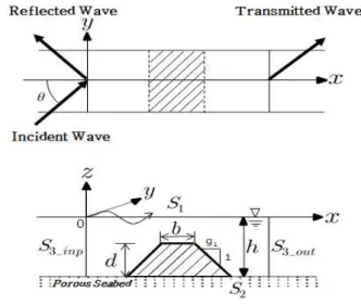
Fig. 1 Analytical Region and Coordinate
2. Basic Equation
2.1 Governing Equation
The submerged breakwater is placed in the water of uniform depth . The axis is directed vertically upwards,
and axis are directed horizontally as shown in Fig. 1.
The incident wave is propagating with an angle to the positive axis. It is assumed that the fluid is inviscid, incompressibility and that its motion is irrotational.
Therefore, the velocity potential can be defined as follows:
(1)
where is the amplitude, is the acceleration of gravity,
is the angular frequency( ). The velocity potential satisfies the following Laplace equation.
(2)
According to the small amplitude wave theory, the velocity potential is given as:
sin cos cos ·
sin cos·
·cosh
cosh
(3)where and are velocity potential at the input and output position, respectively, is the wave amplitude,
and are the unknown variables corresponding to the reflected and transmitted waves and is the wave number.
Since the variation of velocity potential to the axis is expressed as sin within the flow domain, an unknown function meaning the variation of potential is expressed as
in plane, so that the velocity potential on the fluid motion in the flow domains are given as follows:
sin (4)
Substituting Eq. (4) into Eq. (2), Helmholtz equation in terms of the unknown potential function is obtained as follows:
sin (5)
The fluid region is bounded by free surface boundary , porous seabed boundary , and open boundaries
and
.
The boundary conditions in the analytical domain are as follows:
Free surface boundary ;
(6)Porous seabed boundary ;
(7)
Open boundaries
,
;
(8)
where
·
, is an added mass
coefficient, denotes the porosity, is a linear dissipation coefficient, is the normal drawn outwardly on the boundaries, is the exterior velocity potential at the junction of analytical regions, is the soil domain pressure, and is the coefficient of permeability.
The continuous conditions such as mass-flux and energy-flux of fluid motion at each boundary must be satisfied as follow:
Mass-flux ;
(9)
Energy-flux ;
≡ (10)where is the wave pressure component. As an analytical method, the problem for the unknown velocity potential applying Eqs. (6)-(10) can be solved. However the analytical method for the unknown velocity potential must satisfy Eq. (9) and (10) at the junction of each domain because the velocity potential is a discontinuous function.
In this study, the analysis using the wave pressure component as an unknown variable is carried out, in which the wave pressure component is continuos throughout the analytical region. Considering the periodical motion of the incident wave frequency , the wave pressure function is expressed as:
(11)
From Eq. (9) and (10), the velocity potential is defined as follows:
·
· ·
·
(12)
where is . Using Eq (12), each of the boundary conditions can be rewritten as follows:
All domains ;
Free surface boundary ;
Porous seabed boundary ;
Open boundary ;
(13)The open boundary condition can be expressed as follows:
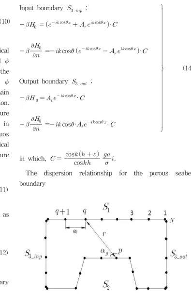
Input boundary
;
cos cos ·
cos cos cos ·
Output boundary ;
cos ·
cos· cos ·
(14)in which,
cos
cos
.
The dispersion relationship for the porous seabed boundary
Fig. 2 Definition of notation
conditions is given as follows(Dean. and Dalrymple, 1984;
Cruz. et al. 1997):
tanh
tanh
(15)where , and is the kinematical viscosity. The dispersion relationship yields a complex valued , which may be written as The real component of represents the real wave number, which is related to the wave length. The is usually small. The has the order of ∼ for sand and has at most for gravel at the normal frequencies.
The theoretical formulation of porous seabed boundary is described in detail (Dean. and Dalrymple, 1984; Cruz. et al., 1997).
2.2 Formulation by Boundary Element Method Let and be two points on the boundaries, and let be the distance between and as shown in Fig.
2; from Green’s second identity, because the velocity potential
is a harmonic function, the following equations are obtained as follows.
sin
(16)where ( ⋯) is the interior angle between two tangents at nodal point as shown in Fig. 2. is the fundamental solution, which satisfies the Helmholtz equation and is defined by the 0second kind Bessel function. When incident wave proceeds perpendicularly, is calculated as ln.
2.3 Formulation about Domain
As shown in Fig. 2, analytical domain is divided with elements and nodal points. The coordinates nodal point of each is denoted by ( …), and the length of each element is ∆ ⋯. The uniform depth input and output boundary and are established at two wave length distance from the structure. The normal velocity vector and the integral direction are counterclockwise. Combining Eq. (16) with Eq. (13), Eq.
(14), and Eq. (15), the following equation is obtained as follow:
·
·
·
(17)
where
,
and
are the arbitrary point on the input and output open boundary, respectively.
3. Validation and Application
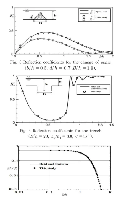
Fig. 3 Reflection coefficients for the change of angle ( ).
Fig. 4 Reflection coefficients for the trench ( , , ).
Fig. 5 Dimension damping coefficient versus depth When an oblique incident wave with incident angle of
, is propagating over an impermeable trapezoidal submerged breakwater, variations of reflection coefficient versus the dimensionless wave length are indicated in Fig.
3. In Fig. 3 solid lines are the results obtained by Ijima et al(1982) using the Domain Decomposition Method, and circle, square symbol are the results obtained in this study.
In addition, in Fig. 4 the reflection coefficients on the trench structure are compared with the result obtained by Kirby and Dalrymple(1983) using the Eigenfunction Expansion Method. Through the comparisons in Fig. 3 and 4, the numerical results obtained in this study agree very well. It shows that this analytical method is verified by validity and availability. Approximated solutions can be obtained from the dispersion relationship, which is plotted in Fig. 5.
(a) Wave profiles on impermeable and horizontal seabed ( )
(b) Wave profiles on porous and horizontal seabed ( )
Fig. 6 Wave profile for oblique incident wave.
Fig. 7 Comparison of energy loss due to incident angle in porous seabed condition ( ).
Fig. 6 shows wave profiles for oblique incident wave in shallow sea water( ). The wave profiles passing on an impermeable and horizontal seabed show the free wave profiles without damping. The wave profiles with damping coefficient under the same conditions in Fig. 6 (a) are damped as shown in Fig. 6 (b).
The energy loss due to porous seabed condition is investigated and presented in Fig. 7. Energy loss has very different value caused from damping coefficient in shallow sea water( ), but energy loss has almost the same value regardless of damping coefficient in deep sea water( ). When the relative depth(=) is bigger than , there is no energy loss, and it may be negligible (Cruz and Isobe, 1997; Dean and Dalrymple, 1984; Reid and Kajiura, 1957). There is no substantial change of the energy loss by the changing of the incident angle.
(a) Horizontal velocities on impermeable seabed ( )
(b) Horizontal velocities on porous seabed ( ) Fig. 8 Comparison of horizontal velocities due to different
incident angle in seabed boundary condition.
Fig. 9 Wave profiles passing over trapezoidal submerged breakwater on impermeable seabed ( )
Fig. 10 Wave profiles passing over trapezoidal submerged breakwater on porous seabed ( ).
Fig. 11 Wave profiles passing over trapezoidal submerged breakwater on impermeable seabed ( ).
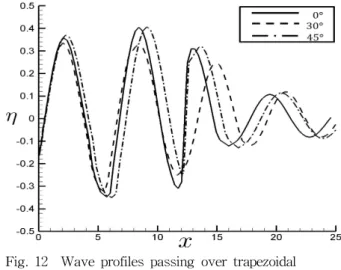
Fig. 12 Wave profiles passing over trapezoidal submerged breakwater on porous seabed ( ).
The horizontal velocities with the oblique incident wave are computed in wave crest and trough as shown in Fig. 8.
is the wave height, is a horizontal velocity in crest, and is a horizontal velocity in trough. The horizontal velocities on the impermeable seabed ( ) including both wave crest and wave trough are greater than those on the porous seabed ( ). When is impermeable seabed, it shows substantial rate of change about horizontal velocities. When is porous seabed, the rate of change on horizontal velocities, because of the energy loss, tends to decrease. Also, Fig. 8 shows that the horizontal velocity due to decreasing incident angle are increased. The numerical results is strong agreement with those of Kim et al (2006).
Fig. 9 and 10 show wave profiles with the oblique incident wave passing on impermeable and porous seabed about trapezoidal submerged breakwater. Fig. 9 shows high wave profiles in front of a submerged breakwater because of reflection due to submerged breakwater, and can be confirmed that wave profiles decrease at behind the submerged breakwater. Fig. 10 shows that the wave profiles over a submerged breakwater on impermeable seabed ( ) are bigger than those over a submerged breakwater on porous seabed( ). This is the evident that wave profiles in front of and at the rear of a submerged breakwater on porous seabed have small value comparing with the wave profiles over impermeable seabed due to energy loss.
Fig. 11 and 12 show the wave profiles over submerged breakwater with the height of , with other conditions same as those in Fig. 9 and 10. Through Fig. 11
and 12, it can be seen that the height of submerged breakwater is higher, wave height is decreasing.
4. Conclusions
In this study, in order to investigate the effect of the submerged breakwater on the oblique incident wave, wave profiles coming with oblique angle to trapezoidal submerged breakwater on the porous seabed were computed by using boundary element method based on the wave pressure function.
The main conclusions from this study are obtained as follows :
(1) When the relative depth() is 0.1 as shown in Fig.
9, 10, 11 and 12, the fluctuation of wave profiles are increased in the rear of the submerged breakwater due to the increase of the transmission coefficient, as the incident angle increases.
(2) When wave is coming with large oblique angle, the wave profile is raised due to the reduction of wave damping rate and the energy loss is decreased in shallow sea water.
(3) In the case of the wave profiles passing on the submerged breakwater on porous seabed, it is able to verify that the attenuation of wave height occurs more significantly due to the wave energy dissipation than that of passing over the submerged breakwater on the impermeable seabed.
Through the results obtained from this study, It is able to prove the effect of a trapezoidal submerged breakwater on the porous seabed. In addition, it is considered to expect more economical and superiorly performable effects of the submerged breakwater through the analysis on the features of real marine and coastal environments.
References
[1] Bai, K, J. (1975) “Diffraction of oblique waves by an infinite cylinder”, Journal of Fluid Mechanics, Vol. 68, Part 3, pp. 513-535.
[2] Chen, K.H., Chen, J.T., Chou., C.R., and Yueh, C.Y.
(2002) “Dual boundary element analysis of oblique incident wave passing a thin submerged breakwater”, Engineering Analysis with Boundary Elements, Vol. 26, pp. 917-928.
[3] Cruz, E.C. M. Isobe. and A. Watanabe. (1997)
“Boussinesq equation for wave transformation on
porous beds”, Coastal Engineering, Vol, 30, pp.
125-156.
[4] Dean, G.R. and Dalrymple, R.A. (1984) “Water Wave Mechanics for Engineers and Scientists”, Prentice-Hall, Inc., New Jersey.
[5] Garrison, C. J. (1969) “On the interaction of an infinite shallow draft cylinder oscillating at the free surface with a train of oblique waves”, Journal of Fluid Mechanics, Vol. 39, Part 2, pp. 227-255.
[6] Ijima T. and Sasaki T. (1971) “Theoretical sutdy on the effect of a submerged breakwater”, Proceedings 18th Japanese Conference on Coastal Engineering, JSCE, pp.
141-147 (in Japanese).
[7] Ijima, T, Yoshida A, Kitayama, H. (1982) “Numerical Analysis on the Reflection Effect of Submerged Breakwater for Oblique Incident Wave”, Proceedings 29th Japanese Conference on Coastal Engineering, JSCE, pp. 418-422 (in Japanese).
[8] Kim, N. H. and Woo, S. M. (2012) “The Boundary Element Analysis of Waves coming with Oblique Angle to a Submerged Breakwater”, journal of the Korean Society of Civil Engineers, KSCE, Vol. 32, No. 5B, pp, 295-300 (in Korean).
[9] Kim, N. H., Young, Y. L., Yang, S. B., and Park, K. I.
(2006) “Wave damping analysis in a porous sea-bed.
Journal of Civil Engineering”, KSCE, Vol. 10, No. 5, pp. 305-310.
[10] Kim, N.H.(1995) “Analysis of the Wave Characteristics of Parallel Submerged Porous Breakwaters by Boundary Element Method”, journal of the Korean Society of Civil Engineers, KSCE, Vol. 15, No. 2, pp.
425-431 (in Korean).
[11] Kirby, J. T. and Dalrymple, R. A. (1983) “Pro pagation of obliquely incident water waves over a trench”, Journal of Fluid Mechanics, Vol. 133, pp.
47-63.
[12] Liu, P.L.-F. and Darymple, R.A. (1984) “The Damping of gravity water-waves due to percolation”, Costal Engineering, Vol. 8, pp. 33-49.
[13] Reid, R.O. and Kajiura, K. (1957) “On the damping of gravity waves over a permeable sea bed”, Transactions - American Geophysical Union, Vol. 38, No. 5, pp. 662-666.
[14] Takikawa, K. and Kim, N. H. (1992) An analytical technique for permeable breakwaters using boundary element method. Engineering Analysis with Boundary Elements, Vol. 10, No. 4, pp. 299-305.
Received 22 March 2013 Revised 13 June 2013 Accepted 13 June 2013