Traffic Classification based on Adjustable Convex-hull Support Vector Machines
Zhibin Yu *, Yong-do Choi**, Gibeom Kil*, Sung-Ho Kim**
조절할 수 있는 볼록한 덮개 서포트 벡터 머신에 기반을 둔 트래픽 분류 방법
1)
위 즈 빈*, 최 용 도**, 길 기 범*, 김 승 호**
Abstract
Traffic classification plays an important role in traffic management. To traditional methods, P2P and encryption traffic may become a problem. Support Vector Machine (SVM) is a useful classification tool which is able to overcome the traditional bottleneck. The main disadvantage of SVM algorithms is that it’s time-consuming to train large data set because of the quadratic programming (QP) problem. However, the useful support vectors are only a small part of the whole data. If we can discard the useless vectors before training, we are able to save time and keep accuracy. In this article, we discussed the feasibility to remove the useless vectors through a sequential method to accelerate training speed when dealing with large scale data.
▸Keyword : Visualization, Traffic Classification, Pattern recognition
요 약
트래픽 분류는 트래픽 관리하는데 중요한 역할을 차지하고 있다. 전통적인 방법은 P2P와 암호화 트래픽을 제대 로 분류할 수 없는 문제가 있다. 서포트 벡터 머신은 기존의 문제를 해결할 수 있고 병목 현상을 극복할 수 있는 유 용한 분류 도구이다. 하지만 서포트 벡터 머신의 주요 장점은 이차 프로그래밍(QP)문제 때문에 큰 데이터 집단을 훈련하는데 시간을 소모한다. 그러나 유용한 서포트 벡터는 전체 데이터에서 극히 일부분이다. 만약 우리가 훈련전 에 쓸모없는 벡터들을 삭제할 수 있다면, 시간을 절약하고 정확도를 유지할 수 있다. 이 논문에서 우리는 대규모 데
∙제1저자 : 위즈빈 ∙교신저자 : 김승호
∙투고일 : 2011. 11. 22, 심사일 : 2011. 12. 09, 게재확정일 : 2011. 12. 28.
* 경북대학교 전자전기컴퓨터학부(School of Electronic and Computer Science, Kyungpook National University)
*** 경북대학교 컴퓨터학부(School of Computer Science and Engineering, Kyungpook National University)
※ This work was supported by the National Research Foundation of Korea(NRF) grant funded by the Korea government(MEST)(No. 2011-0004184).
이터를 다룰 때 훈련 속도를 빠르게 하기위해 순차적인 방법을 통해 쓸모없는 벡터들을 제거하기 위한 가능성을 논 의하였다.
▸Keyword : 시각화, 트래픽 분류, 패턴 인식
I. Introduction
Nowadays, the services provider offers more and more Internet services. Those services bring us much convenience. Meanwhile, various Internet services are coming with a challenge to network management. To offer greater convenience to network management, it is important to investigate and classify the types of network applications that generate user traffic. It’s widely accepted that the well-known ports-based method is inefficient to deal with ever new applications [1][2][3]. In order to support various business goals, operators need to know what is flowing over their networks promptly so they can react quickly.
Commonly deployed IP traffic classification techniques have been based around direct inspection of each packet’s contents at some point on the network. However, Unpredictable (or at least obscure) port numbers are increasingly used many applications [4]. Consequently, more classification techniques correlated with application type by looking for application-specific data (or we called protocol behavior) was developed [5]. However, the effectiveness of such ‘deep packet inspection’
techniques is decreasing. The reasons are simple:
Such techniques need to know the syntax of each application’s payloads while it’s able to inspect the payload of each IP packets.
The challenges come when customers use encryption to protect packet contents (including TCP or UDP port numbers). The governments may also use privacy rules to constrain the ability of third parties to lawfully inspect payloads at all. In fact, many network security services such as signature-based intrusion detection system (for instance, Snort [6] and NFR [7]) and firewall are
widely used in recent years with the growing of the internet traffics.
A number of researchers are looking particularly closely at the application of Machine Learning (ML) techniques (a subset of the wider Artificial Intelligence discipline) to IP traffic classification [8]. Machine learning algorithms are generally categorized into supervised learning and unsupervised learning or clustering.
Support vector machine (SVM) is a set of related supervised learning methods that analyze data and recognize patterns, which is developed based on the statistical learning theory and the principle of the structure risk minimization. SVM has a unique advantage in machine learning field, and soon becomes a fast evolving research topic after it was proposed.
SVM shows a possible way to classify network traffic [9][10]. A main disadvantage of SVM is the training time. The essence of the Support Vector Machine is to solve a quadratic programming (QP) convex problem. The time complexity is O (N3), where N is the number of samples. Based on the work on Joachims [11], the time complexity is close to O (N2). However, the number of input samples N is always large due to the growing traffic flows. As a matter of fact, it causes a heavy load on training step. It’s possible to decrease the training time by decreasing N. But we will lose some accuracy at the same time. It seems that speed and accuracy are always incompatible.
In this paper, we proposed a sequential method
named Adjustable Convex-hull SVM (ACSVM) to
speed up SVM and keep the accuracy. The rest of
this paper is organized as follows: Section II
outlines the theoretical works about our algorithm,
including the basic theory of Support Vector
machine, and discusses the limitations of SVM.
Section III provides our proposed method ACSVM to accelerate the training speed for SVM based on how to select useful support vectors. Section IV shows the experiment result which compares the training time and accuracy between original SVM and ACSVM. Section V concludes the paper with some final remarks and suggestions of possible future work.
II. RELATED WORKS
1. Support Vector Machine(SVM)
Support Vector Machine (SVM) which is a kind of supervised machine learning technology is effective on some alternative situations. An SVM model can be described as points in space, mapped so that the points from two groups are divided by a clear gap that is as wide as possible.
Actually, SVM can be concluded to such an optimization problem:
(1)
where λi and αi is the Lagrange multiplier; ξi is the soft margin; xi is the ith input vector; zi=±1 is the output class of xi; 〈φ(xi),φ(xi)〉 is the kernel function and w is the norm vector to the hyperplane.
This is known as the dual problem. For large data sets, the dual optimization can be solved using numerical techniques (ex. Quadratic programming [12]).
2. Support Vectors
In Formula 1, using the fact of dual form w can be computed as:
(2)
If λi≠0, then xi is so called support vectors.
The support vectors are the training patterns for which Formula 1 represents an equality — that is,
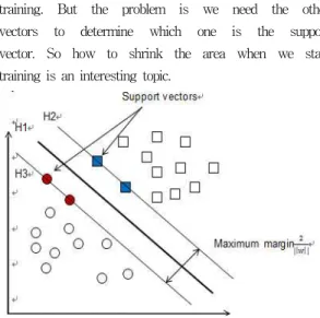
the support vectors are (equally) close to the hyperplane vector (Figure 1). The support vectors are the training samples that define the optimal separating hyperplane and are the most difficult patterns to classify. Informally speaking, they are the most informative samples for the classification task. If we only choose the support vectors to train the hyperplane, of course we could reduce time on training. But the problem is we need the other vectors to determine which one is the support vector. So how to shrink the area when we start training is an interesting topic.
Fig. 1. Training a Support Vector Machine consists of finding the optimal hyperplane. The three support vectors
are shown in solid dots.
Some researches such like ‘Sequential Minimal Optimization’ (SMO) [13], which can greatly reduce the chunk size to 2 vectors, is very useful in linear separable case. In non-separable case, the number of support vectors is much higher than 2. Though we know that most of the support vectors are near by the hyperplane, the problem is, we do not know exactly the position of the hyperplane before training. Some of the algorithms such like SeqSVM [14] showed a kind of solution to decrease the training data as much as we can use the concept of convex hull. But in complex non-separable case, this method is not able to reach the accuracy as high as the original SVM.
For large-scale problems, the dual problem
mentioned in section 2.2.1 will be difficult to
calculate. If we use Quadratic programming, we
have to load a large matrix, so traditional optimization algorithm like Newton method cannot be directly used. Currently one major method for dealing with this problem is to decompose the quadratic programming problem to a sequence of smaller-sized quadratic programming problems which can be solved sequentially[15], [16].
However, for huge problems, especially those with a large number of support vectors, this method needs a large number of iterations and suffers from slow convergence [17]. To find the support vectors in complex situation, random sampling [18] technique is developed based on the idea that the sample near the boundary has higher probability to build the hyperplane. Active Learning with SVM [19]
considers that unlabelled samples are helpful to select the most informative samples for training.
In this paper, we proposed a method named Adjustable Convex-hull SVM (ACSSVM) to speed up SVM and keep the accuracy. And then we use the modified SVM model to classify network traffic.
III. PROPOSED METHODS
1. Adjustable Convex hull
The concept of convex hull mentioned in SeqSVM[14] is the merge of the cross area which only keep the farthest wrong classified sample.
Convex hull SVM Hyperplane
Fig. 2. Convex hull in SVM
Figure 2 shows an illustration of convex hull of a dataset. The yellow samples are so-called convex
hull because such samples are in the periphery area.
Sometimes the information from the convex hull is not enough for us. We may need to adjust the thickness of the convex hull to get more information (The area between two dashed lines.). We called this adjustable convex hull.
Fig. 3. An illustration of convex hull
Figure 3 shows the concept of convex hull in the Support Vector Machines. In the wrongly classified area, convex hull mentioned in [14]
is displayed by colored circles and squares. In another words, samples which satisfy the following formula:
m ax · an d · (3) If zi (w∙φ(xi)) <1 means such output samples’
labels are wrong, and max|w∙φ(xi)| means they have the maximum distance between such sample and hyperplane. These circles and squares have a high possibility to be the support vectors of the whole data. If we only use the colored vectors from convex hull to draw the hyperplane,
there is no doubt that we will increase the training speed and receive a roughly classified hyperplane. But we will lose some useful support vectors at the same time. So our ideal Adjustable Convex-hull model should contain the full information of the wrongly classified area which is displayed by two rectangles in Figure 3. That is equal to increase the thickness of the convex hull.
Finally, we can modify formula 3 to adjust the thickness of convex hull as:
· (4)
where ξi is the soft margin, and t is the thickness
of the convex hull.
Theoretically, the range of t is:
( )
( )
( ) ( ( ( ) ) )
[ z i w x i z i w x i ]
t Î min × j , max × j
If we set t=min(zi(w∙φ(xi))), that means we have the thinnest convex hull which is described in Figure 3. Relatively, we will have thickest convex hull if we choose t=max(zi(w∙φ(xi))). In this case, we choose all of the samples——That is equal to original SVM. Thin convex hull will reduce the calculation time but lose accuracy. Thick convex hull will increase the accuracy and training time at the same time. So the best choice of parameter t may be around 0. In that case, all of the wrongly classified samples will be chosen.
2. Optimal searching process
Suppose a large training set called D = {x1, x2, ..., xn}, where each sample xi is a d-dimensional vector and its label yi∈{+1,−1}, and the distribution of the data sample is unknown. In the ACSSVM, our target is to train the samples which have more probability to be support vectors and pay less attention to the samples which have less probability in the large training set. Initially, ACSVM randomly select a small bit of data from the large training set D. Then, we are able to build the hyperplane H1 based on A and use A to predict D.
Of course the result is not as well as the standard SVM. Next, samples which are in the adjustable convex hull are extracted and added to A. In the second method, more samples will be found and add into A. If we do this step more than 3 times, the accuracy will be much closer to the standard SVM.
Fig. 4. Initializing A form D
In Figure 4, set D consists of squares and circles.
The static color circles and squares which is called A from the former paragraph are selected at the first time randomly,. Based on these randomly selected data A, we are able to make a rough SVM plane H1 at the first step. Then we will check all the dots in D. If one dot is in the adjustable convex hull and it is not in A, add them into A. In Figure 5, we can find the updated A. Then we will enter to the next step: Train A again and draw the hyperplane H2 based on SVM, in this step, compared to H1, ¬H2 will change its orientation and rotate to the other side. In the first two steps, we may find the accuracy is not high if we checked that. Actually, our target in the first two steps is to select most of the support vectors from the adjustable convex hull.
In most of cases, the hyperplane in step 3 (Figure 6) is closer to the one of standard SVM. If needed, we can continue the circulation until the accuracy is no longer changed. But too many steps will waste us a lot of time. We will find the detail experiment results in section 4.2.
Fig. 5. Use A and information of adjustable convex hull from step 1 to draw the hyperplane H2
Fig. 6. In most of situations, step 3 will find the solution which is close to the ideal solution
3. Proposed Algorithm
Supposed there is a large sample D which is consist of two classes called circles as C and squares as S (D=C+S). In Table 1, maxC and maxS are max(zi(w∙φ(xi ))) which is mentioned in Formula 4. PC and PS are the thickness variable which is able to control the depth of the convex hull. If PC or PS > 0, that means we need less depth. This will save time but may reduce the accuracy.
Comparatively, if PC or PS < 0, it will increase the depth of the hull. In this situation, we could receive better accuracy but lose more time. In our experiments, PC = PS = 0.
The flow chart is shown in figure 7. First we need to select a small amount data defined as A from the input data D (ex. 1%) and then use SVM to construct a rough model with mapping function F(x).
By using F(x), we are able to make our first decision and find out the wrong classified data A1. Check each element in A1, if an element from A1 does not belong to A, add it to A and start the next training.
The circulation will be ended if there is no new elements can be found in Ai (i is the number of training times) or the new vectors from Ai are lower than a certain percentage of A (ex. lower than 5%).
Fig. 7. Flow chart
IV. EXPERIMENT RESULT
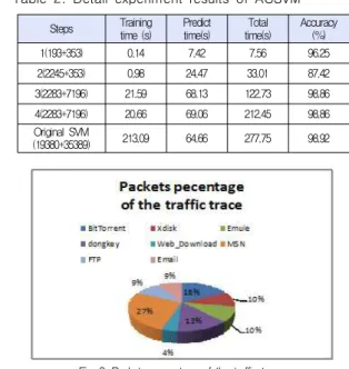
Some large-scale datasets which was based on some traffic flows are used in our experiments.
These traffic flows are captured by Wireshark from our machines. Based on some former research [15], in order to receive the best accuracy, we choose source/destination address, source/destination port, protocol flags and packet size. Hence the data source is a kind of 6-dimensional non-
separable sample. The number of the training samples is from 50 to 508809. We can find that in small scale data case(less than 20000), training time is less than predicting time. That means, if we did too many iterations especially in the later period, we might cost more time than the standard SVM. And what we tried to do is to save training time. So if the scale is too small, it’s not available to use this algorithm.
We tested ACSSVM by using SVM with L2-norm
based soft margin and RBF kernel. LIBSVM
2.8(.NET) was used for SVM algorithm. All
experiments are done by a Pentium 4 3 GHz X 2
machine with 2GB memory. The information of the
whole data traffic is shown in Figure 8. All of the
experiment data is drawn from it.
Table 1. Algorithm (Pseudo codes)
1 Select a small amount of circles and squares randomly as the initial sample A fromD;
2 Use SVM(rough SVM) to train full data sample D based on sample A and get the decision function F(x); //
Supposed if F(x)<0 means circle, while F(x)>0 means squares
3 For each(dot Di in D)
4 {
5 If(Di is in circle C)
6 {
7 if((F(Di)>PC*maxC)&&(Di is not in A))
8 add Di into A;
9 }
10 Else
11 {
12 if(((F(Di)<PS*maxS)&&(Di is not in A))
13 add Di into A;
14 }
15 }
16 If there are no new dots found in step 3~15, terminate.
//( − max min
≦Pc<1, − max min
≦Ps < 1)
1. Increasing time following the number of steps Table 2 shows the detail results in one typical experiment. The percentage of data in this experiment is shown in Figure 8. Although both samples are belong to P2P traffic. In the first two steps, the accuracy is not high. Actually, the result based on the first step is from the initially random data A. So the accuracy may be lower than the result from the original SVM. In the second step, because the new elements from the error classified dots in the first step may be more than the initially data A, the hyperplane(H2 in figure 5) will move to the other side of the ideal hyperplane(H3 in figure 6). This may cause that
the accuracy in step 2 will be lower than the first step. In step 3, based on the updated data sample A, ACSVM will find the solution which will be much closer to the ideal hyperplane than the result of SeqSVM.
Table 2. Detail experiment results of ACSVM
Steps Training
time (s) Predict
time(s) Total
time(s) Accuracy (%)
1(193+353) 0.14 7.42 7.56 96.25
2(2245+353) 0.98 24.47 33.01 87.42
3(2283+7196) 21.59 68.13 122.73 98.86
4(2283+7196) 20.66 69.06 212.45 98.86
Original SVM
(19380+35389) 213.09 64.66 277.75 98.92
Fig. 8. Packets percentage of the traffic trace
In this table, we can find that in step 4, though the number of vectors increased, the accuracy is not changed. That means after 3 steps, most of the support vectors have been found. But in the later period of SCVSVM, time we need to pay will be more than the one in the last time. So it's important to control the steps of the circulation. Although the total times of 4 steps are shorter than the original SVM, in step 4 we lose more than gain. As we considered in section III, if the new vectors from Ai only take a small percentage of A, it would not bring much help to the final decision but waste more time.
2. Advantage of ACSVM
The main cost of SVM algorithm includes two
parts: predict time and training time. The
relationship between predict and training time is
shown in Figure 9. We can find that the prediction
time linearly increases with the number of samples
while the curve of training time approximately
follows an exponential growth. When the number of
samples is larger than 50000, the training time is
several times larger than predict time. In this
situation,
Fig. 9. Relationship between time and training time
training time will dominate the cost of SVM. The motivation of ACSVM is to discard the useless vectors and pick up valuable vectors by sequential training. Although the predict time in each circulation of ACSVM is the same as SVM, it can greatly reduce the training time in each step by only selecting valuable vectors. Because the valuable vectors always take a small part of the whole data, so the training time in each step is much smaller than training with all the samples if the amount of samples is huge enough.
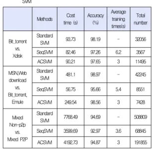
In Table 3, we trained 5 times and use the average value. There is no doubt that both ACSVM and SeqSVM saved time compared to the original SVM. But in complex case, SeqSVM is not able to find most of the possible support vectors. Maybe the precision will be even lower than the random data in first step. From Table 3, it’s obvious that both SeqSVM and ACSVM algorithms are faster than the standard SVM in large scales. In Table 3, ACSVM used only 3 steps. We can find that the accuracy of ACSVM is still better than SeqSVM. In complex case, the accuracy is even better than the original SVM.
Table 3. Comparison between ACSVM, SEQSVM and Standard SVM