46
논문번호17-01-07 http://dx.doi.org/10.7471/ikeee.2017.21.1.46
FastPatch-basedDe-blurringwithDirectional-oriented Kernel Estimation
Kyeongyuk Min
*, Jongwha Chong
*★Abstract
This paper proposes a fast patch-based de-blurring algorithm including kernel estimation based on the angle between the edge and the blur direction. For de-blurring, image patches from the most informative edges in the blurry image are used to estimate a kernel with low computational cost. Moreover, the kernels of each patch are estimated based on the correlation between the edge direction and the blur direction. This makes the final kernel more reliable and creates an accurate latent image from the blurry image. The combination of directionally oriented kernel estimation and patch-based de-blurring is faster and more accurate than existing state-of-the art methods. Experimental results using various test images show that the proposed method achieves its objectives: speed and accuracy.
key words: de-blurring, edge direction, image restoration, kernel estimation, motion blur
.Key words: thermoelectric generator (TEG), dc-dc booster, charge pump circuit, discontinuous conduction mode, low voltage startup circuit
* Dept. of Electronics Engineering,
Hanyang
University★
Corresponding author
e-mail: [email protected] tel: 02-2220-0558
※ Acknowledgment
This research was supported by the MSIP
(Ministry of Science, ICT and Future Planning), Korea, under the Industry4.0s research and development program(S1106-16-1027) supervised by the NIPA(National IT Industry Promotion Agency).
Manuscript received Mar. 29, 2017; accepted Mar. 30, 2017
This is an Open-Access article distributed under the terms of the Creative Commons Attribution
Non-Commercial License
(http://creativecommons.org/licenses/by-nc/3.0) which permits unrestricted non-commercial use, distribution, and reproduction in any medium, provided the original work is properly cited.
1. Introduction
Motion blur is a common artifact cause of disappointing blurry images with inevitable information loss. It occurs because imaging sensors accumulate incoming light over a certain period of time. Unwanted camera movement during exposure makes the sensor take several scenes within a frame, and objects originally captured in designated pixels are placed in unwanted pixels.
If motion blur is , it can be modeled as the
convolution of a latent sharp image with a blur
kernel [1], where the kernel draws the moving
trace of a sensor. Then, motion blur is
removed, in a process called de-blurring that
involves a deconvolution operation. We can
categorize deconvolution into two types by
FastPatch-basedDe-blurringwithDirectional-orientedKernel Estimation 47
existence of a kernel. While in non-blind deconvolution the kernel is provided to recover the latent sharp image, in blind deconvolution, the kernel is unknown and this is more practical model in the real world; therefore we focus on blind deconvolution. In this paper, we focus and propose improvement on the blind deconvolution problem of a
single image where both kernel and latent sharp image are estimated from a blurred image.
Single image blind deconvolution is a well-known ill-posed problem because the number of unknown items (the latent sharp image and the kernel) exceeds the number of given items (the blurry image). Various studies have been performed to address the problem of blind deconvolution for de-blurring a blurred image. Although many researches have tried to recover un-blurred images from blurry ones, aspects of the problem remain challenging. Lokhande et al . [2] have worked on identification of blur parameters using analysis of the frequency domain, and tried to reconstruct the kernel using length and angle information. This method assuming perfect linear kernel might not perform well for natural images. Joshi et al . [3]
estimated the kernel using sharp edge prediction, and tried to predict the ideal edge by searching the local maximum or minimum pixel intensities. This method did not achieve the expected result for large blurs. Levin et al [4-7] proposed an algorithm with image statistics changes of derivative filters by blur, and this provides good results only for box kernels, which represent the characteristics of perfect motion blurs. However, blur is not always motion blurs and most motion blurs do not have perfect box kernels. Fergus et al . [8]
tried to solve the problem by adopting a Variational Bayesian approach to account for uncertainties in the unknowns, allowing the algorithm to find the kernel implied by a distribution of probable images. Shan et al . [9]
usedasemi (MAP) approach to obtain a point
estimate of the unknown quantity based on empirical data. They used a Gaussian prior for natural images and edge re-weighting and iterative likelihood updates for approximation of the latent sharp image. However, this method is not suitable for images that are sparse or not Gaussian. Xu et al . [14] proposed an efficient and high-quality kernel estimation method based on using the spatial and iterative support detection (ISD) kernel refinement and the, TV- l
1deconvolution model, solved with a new variable substitution scheme to robustly suppress noise. Yuan et al . [10] proposed a different system using a pair of images, a blurry image and a noisy image, to reconstruct the latent sharp image.
Bae et al .[11] proposed a novel method that uses mosaic image patches composed of the most informative edges in the blurry image .They reduce computational complexity using patches smaller than the original image. That method generates a small loss in accuracy compared with other de-blurring algorithms due to the limited information in the patches. Moreover, the accuracy of the kernel estimation tends to be affected by characteristics of the patches such as edge direction. However, with progress in the accuracy of patch selection and kernel estimation, this method will be an interesting de-blurring approach in the coming years.
In this paper, we propose a novel kernel estimation method that uses the angles between the edge directions and the blur directions, and we show how this method is suitable for a patch-based de-blurring algorithm.
The rest of the paper is organized as follows. In
Section 2, our motivation for this paper is
analyzed with examples. In Section 3, we describe
the overall algorithm and its core points. In
Section 4, we explain simulated and real data
experiments that show the effectiveness of our
proposed algorithm. In Section 5, we summarize
the proposed algorithm .
2. Motivations
proposed method contains two ideas; the patch-based method and the direction-awareness regularization. In this section we describe other works related to other various regularization terms, and the motivations of the ideas for blur kernel estimation.
2.1 Related work: the regularization term We studied three representative methods with simulation for comparison like; Fergus’s [8], Xu’s [14] and Krishnan’s methods [23].
Fergus’s method in 2006 was earlier study for blind image de-blurring, and its cost function to estimate the blur kernel considered the estimated image, the estimated kernel, and the standard deviation of the gradient histogram of the estimated image as shown below:
2 2
2
( ) ( ) ( )
( ) ( ) ( )
log log log
( ) ( ) ( )
q x q K q
q x q K q
p x p K p s
s s
-
Ñ
Ñ + +
Ñ (1)
where p and q denotes sparsity priors, respectively.<•>
q(-)denotes the expectation with respect to q (-)
2, denotes the standard deviation of the histogram on ∇ x , K represents the blur kernel, and x denotes the estimated sharp image. The standard deviation is the only regularization term, except the kernel and the estimated image, and this was an efficient regularization, while it is not widely used due to low accuracy. Moreover, Fergus’s method used the Richard-Lucy, now considered as an old-fashioned algorithm, for image restoration.
Xu et al . proposed a kernel estimation method using the spatial prior In the kernels estimation step, the cost function is shown below:
2 2
( )
sE k = Ñ x Ä - k y + g k (2)
where x represents the estimated sharp image, k denotes the blur kernel. y denotes the input blurry image, γ denotes the control parameter, and ∇ x
sdenotes the shock filtered gradient image [14].
The regularization term, our focus in this work, is the second term, the square of the absolute, values of the estimated kernel,
2 2( ) s
E k = Ñx Äk - y +
g
kIt prevents a continuous increasing of the estimated kernel, but it does not give any information on the ideal kernel.
Krishnan’s method proposed l 1 norm regularization of the kernel and a nove lregularization of the estimated image, as described in the equation below:
2 1
2 1
2
( , ) x
E x k x k y k
l x j
= Ä - + + (3)
where λ and φ denote the control parameter, and x , k , and y denote the same variables as in the previous method. The regularization terms are the ratio of the l1 norm to the l 2 norm on the estimated image, and the l 1 norm on the estimated kernel. Its ratio increases with blur level and provides information about the blur level. However, the l 1norm on the kernel gives no information either like Fergus’s.
To overcome this shortcoming, we provide an
efficient regularization term for useful information
to the cost function. In this paper, we propose a
directional-derivatives kernel regularization term
for accurate kernel estimation described in
Section 2.3 .
FastPatch-basedDe-blurringwithDirectional-orientedKernel Estimation 49
2.2 Patch-based method
The kernel estimation method we propose is based on the angle between the edges and blur directions. For the same blur direction, the edges on the parallel angle cannot indicate blur information than the edges on the orthogonal angle. Therefore, according to the edge and blur directions, we can reduce the kernel in parallel angle case
In a patch-based algorithm, the region of the patch is much smaller than the full image; thus each patch may contain a partial object with plentiful edge information. As a result, some selected patches include the angle parallel to the blur direction, and others do not have enough information to create an accurate kernel.
This is insignificant when we reference the full image and can uniformly estimate the blur regardless of edge direction. Therefore, this problem has been overlooked in full size image de-blurring, but in the patch-based methods, it is considered as an influential factor for kernel estimation.
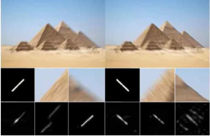
Fig. 1. Example image [Top-left: blurred image with direction 45◦,top-right: blurred imagewithdirection-45◦, middle column: real kernel and two selected patches, bottom column: estimated kernel with whole image and two estimated kernels with each selected patch above.] The kernel estimation is more accurate in the patch orthogonal to the blur direction
Figure 1 shows the significance of our motivation. The simulation image includes a patch with evident direction on both edge and intended blur. We have to pay attention to the
edge direction, the artificial blur direction and their influence on the blurred images and the estimated kernels. The estimated kernels at the bottom of Figure 1 shows that the kernel is accurately estimated only for the patches orthogonal to the blur directions. In the opposite case, many errors generate a severely degraded result. Moreover, the kernels from the orthogonal case patches result in an accurate estimation compared to those from the original full image.
Based on our research concerning orthogonal edges, we concluded we must choose patches with plentiful edge information and uniform distribution of edge direction, to use directional information for kernel estimation.
2.3 Directional derivatives-based kernel regularization
As we explained in 2.2, we considered the direction relationship between edge and blur, and selected patches with enough edges in a uniform direction. After that, we determined how to use the directional information effectively in the blur kernel estimation step.
Our proposal is a novel regularization motivated by Krishnan [23] of a regularization function as the ratio of the l1 norm and l2 norm among the high frequencies of an image.
Regularization in mathematics, particularly in
the fields of machine learning and inverse
problems, refers to a process of introducing
additional information to solve an ill-posed
problem or prevent over-fitting [28]. Therefore,
a reliable regularization term can improve
estimation to achieve an ideal solution. Our
proposal of a direction-based novel regularization
is based on the relationship between blur and
edge directions, which is the core motivation of
this paper.
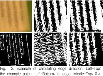
Fig. 2. Example of calculating edge direction. Left-Top:
the example patch, Left-Bottom: its edge, Middle-Top: 0◦
-derivative image, Right-Top: 45◦-derivative image, Middle-Bottom: 90◦-derivative image, Right-Bottom: 135◦
-derivative.
By introducing the proposed regularization into the kernel estimation step, we aim to accelerate an estimated kernel orthogonal to edge direction and decelerate it parallel to edge direction. The proposed regularization term is ∥∂
∥
/ ∥∂
∥
where p represents the parallel to the edge and q represents the opposite. However, p and q are not orthogonal in practice, because each patch contains various edges. (Detail description for selecting p and q is described in below Section2). is the *-direction derivative image of a kernel. ‖-‖
2is the l 2 norm operator.
We described the proposed regularization. The flow is 1) edge direction, p and q selection 2) directional derivatives of kernel, the proposed regularization term.
1) Calculating edge direction
We estimate an edge direction by calculating directional derivatives, as mentioned in Section 2.
Their strengths are calculated by the l 2 norm operation that sums the squares of each directional derivative image. A high l 2 norm score represents the direction orthogonal to the edge, and a low score represents the opposite. Figure 2 shows the examples of images and calculating edge direction. This example patch
has edge directions between 90
◦and 135
◦shown in its edge detected image. Therefore, we expect high norm scores on their orthogonal directions, 0◦ and 45◦. The norm scores of directional derivatives are 1.8141*10
4in 0◦, 1.7976
*10
4in 45◦, 1.4867*10
4in 90◦, and 1.5989*10
4in 135◦, respectively. According to their norm scores, p representing edge direction is selected as 90, because the derivative image along 90◦ has the minimum norm score and q representing blur direction is selected as 0◦.
We want to make it clear that blur direction does not describe the actual motion of the blur;
direction of blur as used in the kernel estimation step is more reliable than other definition.
2) Directional derivatives of the kernel
By calculating the edge direction mentioned in 1), we decided which direction of the blur kernel should be emphasized. The detailed description of the word, ‘emphasized’, is that the blur kernel along the designated direction influences an estimated kernel in the next iteration. To do this, we should assign a high regularization score on the direction parallel to edge and a low score on the orthogonal in the cost function of the kernel estimation step.
In the proposed regularization term, we used the
l 2-norm score on the directional derivatives of the
estimated kernel. It can represent the direction of
blur kernel: a low score denotes direction parallel
to the filter, and a high score denotes the
orthogonal direction as shown in Figure4. We are
convinced that the l 2 norm scores can be used as
a regularization term because they vary with
regard to the blur direction; they are directly
proportional to the distance between the filter
direction and the blur kernel direction (the
distance between 137◦ and 0◦ is considered to
be 43◦, not 137◦; 0◦ can be considered
equivalent to 180◦).
FastPatch-basedDe-blurringwithDirectional-orientedKernel Estimation 51
We selected the parallel direction p , and the orthogonal direction q by using the l 2 score of patches. After that, the proposed regularization term is directly proportional to the l 2 norm of the directional derivative along p and inversely proportional to it along q , expressed as
Fig. 3. Artificial blur kernels along direction 0◦to170◦
withstepsize10◦.
Fig. 4. l2-norm scores with the directional filter.‖∂
*‖
The x-axis represents the degree of the artificial blur kernel, and the y-axis represents the l2 norm scores. For the artificial blur kernels in Fig.3, we applied the directional filters discussed in Section3. Along all directions, l2 norm scores have the minimum score on the direction parallel to the filter and the maximum on the orthogonal.
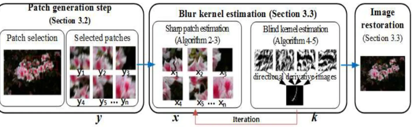
Fig. 5. Flow of the proposed algorithm. We selected informative patches and kernel estimation with iteration between sharp patch estimation and blind kernel estimation. With the estimated kernels, we restore the sharp image
.
.
3. Proposed Method
3.1 Overall algorithm
We assume the formulation model of a latent sharp image x blurred by a kernel k along with the addition of Gaussiani.i.d noise n . This is representedas as Equation 4.
,
y = k Ä + x n (4)
where y is the observed image and our goal is to recover the unknown sharp image x and the kernel k . In general, variables are inserted into the cost function, and iterations are performed to minimize the energy function in terms of x and k .
In this paper, we use a patch-based de-blurring method to estimate the kernel k , and to recover the latent sharp image x . Patch-based methods use the same formulation model, however x , y , and k represent each kernel and the final estimated kernel is applied to the full-size observed image for recovery.
Figure 5 outlines our proposed method.
Section 3.2 explains the construction of edge informative maps and the algorithm that finds a set of patches that cover all possible edge-orientation angles and is likely to be informative in estimating image blur.
In Section 3.3, we describe the proposed estimation method for the kernel with the novel directionally-oriented step. In this step, we describe how the directionally-oriented method is used to estimate the kernel. In Section 3.3-1), we show the method for approaching the latent sharp image using the estimated kernel from Section 3.3-2). Section 3.3-3) describes a non-blind image restoration using the estimated kernel from Sections 3.3 1) and 2).
Fig. 6. Representation of the direction four groups. [j = 0, 45, 90, 135]
3.2 Image Patch Selection
Our original patch selection objective was only to reduce the amount of data without losing accuracy. As mentioned in several papers, edge information found in the observed blurry image is useful for estimating the kernel. Several important characteristics of edges, including the, gradient magnitude, orientation angle, width, and straightness [3-16], are widely used in state-of-the-art blur-related methods. Traditional de-blurring approaches apply masks on top of the observed blurry image to build the kernel estimation algorithm and focus on the most informative region in the blurry image.
Therefore, the main objective of these approaches is not only to reduce computational complexity, but also to use informative edges.
Several previous methods require user intervention to choose the optimum region, which is thus determined by the human visual system instead of mathematical calculation. A region might look like the most informative region when in fact it is not. Therefore, user intervention reduces accuracy. On the contrary, we determine the informative patches within the blurry image using mathematical equations for characteristics, edge strength [17] and uniformity of edge direction.
Motivated by the structure of the edge strength used in [17] for image quality assessment,
[ j = 0 ]
{θ | -22.5 ≤ θ <22.5 and 157.5≤ θ <202.5}
[ j = 45 ]
{θ | 22.5 ≤ θ <67.5 and 202.5≤ θ <247.5}
[ j = 90 ]
{θ | 67.5 ≤ θ <112.5 and 247.5≤ θ <292.5}
[ j = 135 ]
{θ | 112.5 ≤ θ <157.5 and 292.5≤ θ <337.5}
FastPatch-basedDe-blurringwithDirectional-orientedKernel Estimation 53
we propose a directional edge strength map and uniformity map described as follows.
Denote the observed blurry image as
[ , , , ,
1 i N]
N,
y = y L y L y Î R (5)
where i indexes the pixels and N denotes the total number of pixels. The local pixel
regularity of the image along multiple directions is measured by directional derivatives represented by.
_ { | var[ (
_)] }, _ arg max( )
m j
i u
i j i j
E U i y T
m j y
h
¬ ¶ <
= ¶ This denotes the directional derivative at the i
thpixel along the direction indexed by j.
We consider only four directions for simplicity (Fig.6), namely,j=0,45,90 and 135. The directional derivative
_ { | var[ (
_)] }, _ arg max( )
m j
i u
i j i j
E U i y T
m j y
h
¬ ¶ <
= ¶ , i =1,2,…, N are computed by convolving y with the directional
high-passfilter F
j, j =0,45,90,135,as described by Equation(6):
0 45
90 135
0 0 0 0 0 0 0 3 0 0
0 3 0 3 0 0 0 0 10 0
1 1
, ,
0 10 0 10 0 3 0 0 0 3
16 16
0 3 0 3 0 0 10 0 0 0
0 0 0 0 0 0 0 3 0 0
0 0 0 0 0 0 0 3 0 0
0 3 10 3 0 0 10 0 0 0
1 1
0 0 0 0 0 , 3 0 0 0 3
16 16
0 3 10 3 0 0 0 0 10 0
0 0 0 0 0 0 0 3 0 0
F F
F F
é ù é ù
ê - ú ê ú
ê ú ê ú
ê ú ê ú
= - = -
ê ú ê ú
- -
ê ú ê ú
ê ú ê - ú
ë û ë û
é ù é
ê ú
ê ú
ê ú
= = -
ê ú
- - - -
ê ú
ê ú -
ë û
, ù
ê ú
ê ú
ê ú
ê ú
ê ú
ê ú
ë û
(6)
The strength map and uniformity of edge direction map are derived using the four directional derivatives.
First, for the strength map, it should be noted that regularity along the edge direction and irregularity along its orthogonal direction together imply the possibility of an edge. In other words, edge strength is defined by two directions in the diagonal and vertical-horizontal because we assume that the edge directions are simplified into four directions. This approach can distinguish edges with a sharp pixel change and the anisotropic structures of image edges.
The edge strength in the diagonal directions is described as follows;
(0,90) 0 90
_
i i i p,
E S = ¶ y - ¶ y (7)
where p is introduced to nonlinearly rescale the edg estrength. The l
2norm is used in this paper. In the same way, the edge strength in the vertical-horizontal direction is defined as follows
(45,135) 45 135
_
i i i p,
E S = ¶ y - ¶ y (8)
The final edge strength map is determined along the stronger direction like the human visual system.
(0,90) ( 45,135)
_ { | max[ _
i, _
i]
s},
E S
¬
i E S E S>
T(9) where E _ S represents the strong edge strength points, and T
sis the threshold that is the total mean in the full image.
Second, the uniformity of edge direction means that the points of the edge are evenly distributed along a similar direction; thus the influence of each edge is no more powerful than that of the other edges. Therefore, under the uniformity condition, the blurring movement of each point can be preserved enough to estimate an accurate kernel. In the calculation of the uniformity of edge direction, the directional derivatives are as follows:
_ { | var[ (
_)] }, _ arg max( )
m j
i u
i j i j
E U i y T
m j y
h
¬ ¶ <
= 
(10)
where E_U represents points of uniformity, represents the neighboring pixels based on i with a size of 3 or 5 in this paper, T
uis the threshold set to the total variance in the full image, j is selected among the four directions,[0,45,90,135],which has a maximum
_ { | var[ (
_)] },
_ arg max( )
m j
i u
i j i j
E U i y T
m j y
h
¬ ¶ <
= ¶ value on pixel I. and var symbolizes the variance operator. We derive the uniformity of edge direction from the directional differences between neigh boring pixels.
We merge the edge strength and the uniformity maps into a final patch map with the between the two map:
_ { | _ _ },
patch map ¬ i E S Ç E U (11)
where patch_map represents the candidate points for patch windows in the observed blurry image.
To create windows within the scattered points on the patch map, we apply an improved K -means clustering method with reduced computation cost [18-22] that clusters the scattered points as described in Figure 7. Due to the clustering method and the process of the final patch map, there is little increase in the computational costs; however, we used the fast K -means clustering method, which takes about 0.14seconds for K =9 [22].
With the kernel estimation in the next step, we can reduce the computational cost by about ( number of patch * patch_size ) / full_image_size, which is around 1/10 or less.Patch size is determined based on the kernel size; however, it is varied by comparing the number of elements in each cluster.
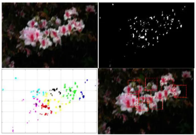
Fig. 7. Overview of the patch selection method, from left to right an top to bottom: the observed blurry image, the final patch map, the clustered patch map using K-means clustering and the final selected patch marked with a red rectangular window. We can see that the proposed method selects the informative region with enough edges.
3.3 Blind Blur Kernel Estimation
Our kernel estimation approach is performed with several selected patches, which means the algorithm refers only the selected patches instead of the whole image to reduce the computational complexity.
Our blind kernel estimation is motivated by Krishnan’s method [23], which proposed a new type of image regularization requiring the lowest cost for a true sharp image. We propose an algorithm based on this and introduce a directionally oriented approach on the kernel estimation step.
Given the observed blurry, noisy input y, the directional derivatives ,
_ { | var[ (
_)] }, _ arg max( )
m j
i u
i j i j
E U i y T
m j y
h
¬ ¶ <
= ¶ , i = 1, 2,…, N are computed by convolving y with the directional high-pass filterF
j,j=0,45,90,135 mentioned before.
In Section 3.2 we used i -notation as a pixel number; however from here forward, we consider i as the patch number. N represents the number of patches. We express the cost function for spatially invariant blurring as:
2 1 2
2 1
, 1
2 2
min
i
i p N j
j j
i i j q
x k i j
x k
x k y k
x k
a b y j
=
é ¶ ¶ ù
ê ¶ Ä - ¶ + + + ú
¶ 
ê ú
ë û
åå (12)
where x and
yrepresent the directional
derivatives along four directions of the un-known
sharp image and the observed blurry image,
FastPatch-basedDe-blurringwithDirectional-orientedKernel Estimation 55
2 1 2
2 1
, 1
2 2
min
i
i
j p N
j j
i i j q
x k i j
k x
x k y k
x k
a b y j
=
é ¶ ¶ ù
ê ¶ Ä - ¶ + + + ú
¶ 
ê ú
ë û
åå
_ { | var[ (
_)] }, _ arg max( )
m j
i u
i j i j
E U i y T
m j y
¬ h ¶ <
= 
and represent the directional derivative of the i
thselected patch along
j-directionwherej∈{0, 45, 90, 135}, and ∂*represents the directional derivative kernel along the individual direction of p
ior q
i, where k describes the un-known kernel with k ≥0, ∑k
= 1. α , β , ψ , and φ are scalar weights to control the relative strength of regularization terms, and the ∥∥
1and ∥∥
2operators represent l
1norm and l
2norm operations.
The cost function, Equation (12), consists of four terms based on Krishnan’s method [23].
The first term takes into account the formulation described in Equation (4) representing the difference between the estimated image with the estimated kernel and the observed blurry-noisy image. It reaches its minimum with an accurately estimated image and kernel. The second term is the l
1/l
2regularization of the x term. It encourages scale-invariant sparsity in the reconstruction.
The third term is the regularization of the kernel, which suppresses the noise in the estimated kernel. The fourth term is proposed in this paper: ∂ and ∂ are the directional derivative kernels along the individual patch directions p
iand q
i, where p
irepresents the angle with the minimum edge strength and q
iis the angle with the maximum of the i
thpatch in Equation(9).
With the non-convex cost function in Equation (12), we search for the best combination of the sharp image x and the kernel k. The search starts with an initial x and k and then iteratively alternates between x and k updates, with the search algorithm reducing iterations and avoiding local minima by introducing conventional efficient minimization algorithms.
The initial x and k are the observed blur image as the initial x and the 3-by-3 matrix filled with the cross shape,[010;111;010],as the
initial k , respectively.
1) Sharp Image x-Update
The sharp image restoration is based on Krishnan’s method [23]. The cost function for updating x is as below:
(13)
With the presence of the regularization term
l1/l
2, Equation(13) can be solved by a minimization algorithm. We chose ISTA, the iterative shrinkage-thresholding algorithm by Beck [24]. ISTA can be considered an inverse transform, which estimates a sharp image from a blurry image and kernel. The basic formulation of ISTA is as follows:
2
min
1x
a Ax b - + b x
(14)
We can substitute k for A and y for b; k and
y,mentioned in Equation (13) and (14) for solving Equation (13) using ISTA method. The core difference exists in the second term, l
1/l
2and l
1. To solve Equation (13) using ISTA, the
l2term is considered the constant dominator of the regularizer. Therefore, the l
2term, ∥
x∥
2, is calculated from the previous iteration and fixed at one iteration. The ISTA step is used as the inner iteration for updating x, and the outer loop simply re-estimates the weighting by updating the denominator ∥
x∥
2. The overall algorithm is described in Algorithm 1and 2.
2 1
, 2
1 2
min
N j
j j
i i j
x k i j
x k y x
a b x
=
é ¶ ù
ê ¶ Ä - ¶ + ú
ê ¶ ú
ë û
å å
Algorithm 1: x-Update Algorithm Assume: Kernel kfrompreviousk-update
Image x
0frompreviousx-update Regularization parameter
α = 20Maximum outer iterations M=2 Maximum inner iterations N=2 ISTA threshold t=0.001
1 for j = 0 to M-1 do2 α’ = α∥xj∥2
3 xj+1 = ISTA(k, α’, xj,t,N) 4 end for
5 return Update imagexM
Algorithm 2: ISTA Assume: Operator k, kernel
Regularization parameter α, Initial iterate x0 Observed image y,Thresholdt
Maximum iterations N Soft shrinkage operator S*
1 for j=0toN-1do 2
v=x
j–tk
T(kx
j-y)
3x
j+1=S
βt (v)j4 end for
5 return Output image xN
*
sgn( ) : 01 001 0
( ) max( , 0) ( )
t i i i
if v
v if v
if v
Sb v v bt sgn v
- <
= =
>
= -
ì í î
2) Blur Kernel k - Update
The method used for updating the kernel is based on the proposed directionally-oriented method that uses the relationship between the edge direction and the blur direction. This relationship is used in the regularization term of the cost function for the updating kernel. In detail, the regularization term consists of two variables: the kernel following the angle with the strongest edge strength, and the kernel following the angle with the weakest. The two variables compose a fraction with the kernel on the strong edge as the denominator and the other goes to the numerator. On the way to the optimal minimum of the cost function, the algorithm tries to reach a smaller regularization value by increasing the denominator, (the kernel
on the strong edge direction image), and decreasing the numerator, (the kernel on the weakest edge direction image).
Therefore the final kernel includes more information in the strongest edge direction.
The cost function for updating k is described in Equation(15).
2 2
2 1
, 1
2
min
i
i N p
j j
i i q
x k i j
k
x k y k
a y j k
=
é ¶ ù
ê ¶ Ä - ¶ + + ú
ê ú
ë û
åå
(15) subject to the constraints k≥0and,∑
iki= 1.∂
and ∂
are the directional derivative kernels along the individual patch directions p
iand q
i, wherep
irepresents the angle with the minimum edge strength and q
iis the angle with the maximum of the i
thpatch. To recapitulate
the patch-based method, the kernel estimation considers not the whole image but N selected patches. To prevent the denominator from becoming zero, we replace the zero-denominator with 1 max (∥∂ ∥
2,1).
Minimizing the cost function to estimate the blur kernel requires a different search algorithm from the x-update. The iterative reweighted least square (IRLS) and conjugate gradient (CG) methods are generally used to update k in the various de-blurring methods. During the iteration, the IRLS with CG method approaches the optimal kernel with updating weights from the previous iteration, and the directional kernel shown in Equation (15). The outer loop is based on the CG method and the inner loop for weight generation is based on the IRLS, as described in Algorithms 3,4, and 5
FastPatch-basedDe-blurringwithDirectional-orientedKernel Estimation 57
Algorithm 3: k-Update Algorithm Assume: Kernel k from previous k-update
Image xfrompreviousx-update Observed image y
Maximum outer iterations M1=2 1 for i = 0 to M1do
2 weights_k = ψ *l1(k)+φ*[l2(kp)/l2(kq)]
3 k_opt = kernel_optimization(k,x,y,weights_x,M2) 4 end for
5 return Update kernelk_opt Algorithm 4: kernel_optimization
Assume: Kernel k frompreviousk-update Image x from previous x-update Observed image y
Maximum inner iterationsM2=2
Weights from outer loop
weight_k
1 Ak = weight_generation(x,k,weight_k) 2 r0 = y–Ak
3 for iter = 1 to M2do 4 rho = (riter)T*riter
5 if iter > 1 do
6 Βiter=rho/rho_prev
7 ziter=riter+Βiter*ziter-1
8 else ziter=r0
9 end if
10 weights_p=ψ*l1(k)+φ*[l2(kp)/l2(kq)]
11 Ap = weight_generation(x,p,weights_p) 12 Αiter=rho/[(Ap)T*(Ap)]
13 kiter=kiter-1+Αiter*ziter
14 riter= riter-1-Αiter*Ap
15 rho_prev=rho 16 endfor
17 return kiter
Algorithm 5: weight_generation
Assume: Kernel k from previous k-update Image xfrompreviousx-update Weights from outer loop weight_p 1 cost = conv(conv(x,k),rot180(x)) 2 final_cost = cost+weight_p*k 3 return final_cost
rot180(A) rotates the matrix A through 180 degrees
During kernel updating, the most important issue is an excessive number of iterations which makes a process slow. Therefore a multi-scale estimation using a coarse-to-fine pyramid of image resolution to reduce computational cost is applied to the implementation [23]. It means that the kernel size is gradually increased from initial to a user-defined size. An initial kernel, as a coarse level, is a 3-by-3 matrix filled with a cross shape, k
init=[010;111;010]. We gradually increase its size with a ratio of until it reaches a user-defined kernel size.
3) Image Restoration
In the final image restoration step, we have the estimated kernel and the blurry image; thus the original restoration problem is transformed into a non-blind image deconvol-ution problem. In this case, we find a target sharp image based on the method of [27] because it is conceptually simple and yields high quality results. The core difference is that they use bi-directional filters and we use four directional filters, in Section 2 like below:
2
1
min ( ) ( )
N
m
i i
u i m
x k y y F
aa
=
æ ö
Ä - + Ä
ç ÷
è ø
å å
(16) where x represents the target sharp image we want to estimate, k describes the final estimated kernel and y show the observed blurry image. F
mis the directional derivatives filter along the
m-direction, m=0,45,90,135respectively.αcontrols regularization weights, used as 1/4or1/3.
4. Simulation Results
Our method contains novel approaches to image
patch selection and kernel estimation. To show
the effectiveness of our method, we began with
a patch selection simulation. The second
simulation demonstrated the effectiveness of the
kernel estimation by comparing the estimated kernel and the expected kernel.
Additional simulations were conducted to show the performance of our method on various images. We implemented our method in MATLAB 2013 on an Intel Core i7-3770 CPU with 16GB RAM on 64-bit Windows 7. The comparison simulations used the algorithms of Fergus, [8]
1, Xu [14]
2, Krishnan [23]
3, and Lin [30]
4their code are distributed for educational research on the cited websites.
Fig. 8. Comparison between developers’ suggested patches and the patch locations selected by the proposed method: patches on the left images were suggested by the developers and the patches on the right images were selected by the proposed method. Their kernels were calculated by Fergus’s method to compare the efficiency of patch selection.
4.1 Simulation Results of the Patch Selection Method
We performed two types of simulations: One compares results between the patches suggested by earlier developers and those selected by the proposed method (Figure 8).
The second simulation shows the performance of the patch selection method on various kinds of test images (Figure 9).
In Figure 8, we compare one patch selected with our method with Fergus’s patch [8] that ensures best performance and estimated the kernels using the method in [8] to unify kernel estimation. The selected patches contained regions similar to the suggested patches, and their kernels were also similar. This indicates that proposed method without human intervention preserved the accuracy of kernel estimation.
The second simulation of the patch selection method showed that the selected patches for various test images can be used widely in de-blurring simulations. There were no right answers for the patch locations. However, we considered the regions with information-rich edges and unified edge directions as reliable patch regions. Figure 9 shows that the proposed patch selection gives credible results.
The number of patches, N, can be fixed to eight. However, N varies adaptively per image.
Fig. 9. Patch simulation. From top to bottom, building,
Roma and boat shown in [11]. The right sides of the
blurry images are k-means results of the patch maps,
and sub-images under them are the selected patches.
FastPatch-basedDe-blurringwithDirectional-orientedKernel Estimation 59
4.2 Simulation Results of the Kernel Estimation Method
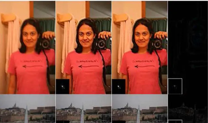
We organized the simulated environment as follows: the kernel estimation algorithm is the modified variable, the image reconstruction algorithm is the control variable, and the estimated kernel and the estimated sharp image are the dependent variables. We used x-update and Krishnan’s method for image reconstruction in both simulations, and Krishnan’s method fo rkernel estimation [23] for comparison with the proposed algorithm. We can prove the effectiveness of the proposed kernel estimation by comparing the estimated kernels and reconstructed images. We did not include a patch selection step to control all variables except the kernel estimation algorithm. In Figure 12, the first and the second rows of images were processed with the optimized parameters suggested by [23], and the parameters of the third image were hand-tuned by iterative simulation. Common environments are that the inner and outer loop iteration for x -update are 2, and the number of iteration between x and k updates is 21. The dependent variables are that the regularization parameters of the x-update are 190 in the first row, and 150 in the second row. Figure 12 shows that the proposed method proceeds in a way similar to Krishnan’s method, but it also shows that the results of the proposed method provided clearer images than Krishnan’s method.
For example, the text on the woman’s top in the first row is clearer in the third .column than in the second column. In the second row, the result in the second column might look clearer than the result in the third column;
however, the result in the second column actually has more rising artifacts because of immoderate enhancement near the edges . Moreover, they evidently described that the proposed method could attenuate the kernel along edge direction: the kernel along vertical was removed in the proposed result.
4.3 Simulation Results of the Proposed Method
To demonstrate the efficiency of the proposed method in both of the above steps and as a whole, we simulated a blind image deconvolution with widely published test images from de-blurring studies and real-captured images to compare our results with several state-of-the-art methods: Fergus [8], Xu [14], Krishnan [23]. For the simulations, we used MATLAB codes or executable files distributed by the authors on their web sites and their parameters for each images were hand-tuned to produce the best results. Likewise, the kernel sizes of each image were fixed according to optimized results of the state-of-the-art methods. In case of [8], the number of non-blind deconvolution was set to 20, the number of kernel estimation iteration was set to 'kernel_size / sqrt(2)'. In case of [14], they blocked the user-intervention to modify parameters. In case of [23], λ were fixed to 50, 90, 90 and 30 at first to fourth column images. φ was fixed to ‘kernel size*(3/13)’ as mentioned in that paper. The number of iteration at coarsest level was 21. In case of the proposed method, α were 40, 70, 70 and 50 at first to fourth column images. β was fixed to 1.3, ψ was fixed to ‘kernel size
*(1/13)’, and φ was fixed to ‘kernel size
*(2/13)’. The number of iteration at coarsest level was 21 same with [23].
In Figure 13 we show the simulation results
for four test images processed by the four
different methods. They demonstrates that the
proposed method reconstructs the observed
blurry images into sharp images with a level of
sharpness similar to that found with the
conventional methods. Advantages of the
proposed method are that the ringing artifacts
near edges are quite reduced, and the details of
objects are well preserved. With comparing to
Xu’s method, the results of the proposed method
look better at third and fourth images, however,
the result images at first and second image look worse than them. Therefore, we simulated the objective evaluations with four methods in Section.4.4 to verify the performance of them.
4.4 Simulation Results of the Proposed Method With Artificially Blurred Images To further demonstrate the performance of de-blurring algorithms, we simulated with artificially blurred images. With sharp test images distributed by the Eastman Kodak Company
5, we applied artificial blur. Therefore, we could measure objective results which need the original and the comparison target images, such as peak signal to noise ratio (PSNR) and structural similarity (SSIM) [25] described in below.
1 2 1 2
1 2 1 2
1 2
1 2 2 2 2 2
1 2
(2 )(2 )
( , )
( )( )
I I I I
I I I I
c c
SSIM I I
c c
m m s
m m s s
+ +
= + + + + (17)
where
I1and
I2represent the average values of
I1and I
2.
1 2 1 2
1 2 1 2
1 2
1 2 2 2 2 2
1 2
(2 )(2 )
( , )
( )( )
I I I I
I I I I
c c
SSIM I I
c c
m m s
m m s s
+ +
= + + + and +
1 2 1 2
1 2 1 2
1 2
1 2 2 2 2 2
1 2
(2 )(2 )
( , )
( )( )
I I I I
I I I I
c c
SSIM I I
c c
m m s
m m s s
+ +
= + + + represent the variance + values of I
1and I
2.
I1I2draws the covariance of
I1and I
2.
=
and
=
are two variables that stabilize division with a weak denominator, where L is the dynamic range of the pixel values (2
*bits), k
1is set to 0.01, and k
2is set to 0. Moreover, we measured the simulation times.
We constructed the simulation environments: the test images were ‘baboon’, ‘cameraman’, ‘lena’
and the selected Kodak images numbered as ‘01’,
‘06’, ‘14’, ‘17’, ‘19’ and ‘24’, shown in Figure 10.
The artificial blurs shown in Figure 10 were generated by the blur effects of MATLAB 2013 with the kernel size fixed to 35x35.
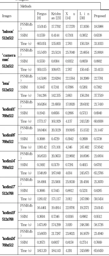
We implemented our methods and simulated in MATLAB 2013 on an Intel Core i7-3770 CPU with 16GB RAM on 64-bit Windows 7. Table 1 shows that the simulation results: PSNR, SSIM scores and simulation times. Note that the Fergus, Krishnan and the proposed method were simulated on the MATLAB 2013 and Xu was
simulated on the C++ program which is faster than the MATLAB language about 500 times [29]. Because Xu et al . only distributed the software as C++. Therefore we have to consider the different simulation environment cause of software. The number of patches of the proposed algorithm were fixed as 4 on 512x512 and 6 on 768x512, respectively. Their patch size was fixed as 100x100. The other methods used the whole-image.
Table 1 described that the proposed method achieved the high quality results with shortened time. With regards to the accuracy, we compared the PSNR and SSIM scores: the proposed method averagely increased 138.41%, 106.67%, 102.75% and 121.66% in PSNR, 235.90%, 116.68%, 105.60% and 145.23% in SSIM comparing to Fergus, Krishnan, Xu and Lin’s methods respectively. The simulations of
‘kodim14’, ‘kodim17’ and ‘kodim24’ showed that the Xu’s method had little higher accuracy than the proposed. Because their kernels except
‘kodim17’ had Gaussian distribution whose directions were uniformly allocated. In terms of the speed, we expected the reduction about the ratio of patches over whole image size and the additional times for patch selection. The processing times of the proposed method were reduced to 4.05%, 32.76%, 1437.58% and 24.37%
(sum of processing times of proposed results /
sum of processing times of their results),
comparing to Fergus, Krishnan and Xu’s
methods, respectively. As mentioned before, if
we consider that Xu was implemented as the
C++, the ratio between Xu and the proposed
can be considered as 2.87 %.
FastPatch-basedDe-blurringwithDirectional-orientedKernel Estimation 61
Methods
Images Fergus
[8] Krishn an [23] X u
[14] L i n
[30] Proposed
‘baboon’
512x512
PSNR(db
) 15.0145 17.7792 17.7270 17.1056 18.5988 SSIM 0.1559 0.4144 0.7101 0.3852 0.6338 Time (s) 663.051 135.003 2.783 150.318 33.1033
‘camera man’
512x512
PSNR(db
) 15.5470 23.5124 25.7040 21.6654 25.9918 SSIM 0.5550 0.8304 0.9352 0.8059 0.8902 Time (s) 950.155 109.871 2.767 150.445 33.4153
‘lena’
512x512
PSNR(db
) 14.5186 22.6284 22.1564 18.2089 22.7781 SSIM 0.3447 0.7241 0.7096 0.5261 0.7362 Time (s) 744.296 142.335 2.663 156.204 37.7519
‘kodim01’
768x512
PSNR(db
) 16.6264 21.6950 17.0920 20.6192 21.7410 SSIM 0.1943 0.6656 0.2896 0.5713 0.6940 Time (s) 1773.17 161.929 4.137 243.520 60.0938
‘kodim06’
768x512
PSNR(db
) 18.0404 20.3129 19.9185 15.1532 21.1447 SSIM 0.3688 0.4729 0.3942 0.2699 0.5738 Time (s) 1383.42 171.101 4.346 247.402 57.9542
‘kodim14’
768x512
PSNR(db
) 16.8533 20.3653 22.9692 18.8586 21.6834 SSIM 0.2492 0.5179 0.7281 0.4015 0.6792 Time (s) 1548.89 187.840 4.034 245.873 65.2706
‘kodim17’
512x768
PSNR(db
) 18.4991 23.5001 25.9530 20.4591 25.3070 SSIM 0.3666 0.7445 0.8812 0.5231 0.8285 Time (s) 1281.02 171.117 3.912 247.090 59.5454
‘kodim19’
512x768
PSNR(db
) 16.4461 19.4914 22.9791 19.2371 23.0145 SSIM 0.3604 0.7346 0.9316 0.8962 0.9512 Time (s) 1473.89 174.299 3.920 248.306 58.1726
‘kodim24’
768x512
PSNR(db
) 15.6670 21.7287 23.8021 16.1679 23.4940 SSIM 0.2673 0.6837 0.8158 0.2714 0.7669 Time (s) 1813.20 184.143 4.201 243.689 65.6450
Table 1. De-blurring results with various artificially degraded
images.
Fig. 10. test images and their artificial kernel used for artificially de-blurred simulations described in Table 1:
‘baboon’, ‘cameraman’, ‘lena’, ‘kodim01’, ‘kodim06’,
‘kodim14’, ‘kodim17’, ‘kodim19’ and ‘kodim24’. Bottom line is the artificial kernels applied to each images in sequence.
The proposed method consists of three steps:
patch selection, kernel estimation and non-blind image restoration. Comparing to the other method, we reduced the time for kernel estimation by using a few selected patches and maintained the time for non-blind image restoration, because it used the whole image and the estimated kernel. . Figure 11 shows the proportion of the processing time, calculated by the average of each steps on various images.
Fig. 11. The proportion of the processing times: the patch
selection step, the kernel estimation step and the image
restoration step
5. Conclusion
In this paper, we proposed a novel image deconvolution method to remove blur from a single image by minimizing errors caused by unintended camera motion. Our main contributions are an effective cost function of the kernel estimation that accounts for its directional correlation, and a reliable patch selection to reduce computational complexity These two methods interact with other traditional methods to improve restoration of the observed blurry image.
In summary, the proposed algorithm first selects patches based on edge strength and edge uniformity along four directions. After that, with selected patches as whole image, the kernel estimation step and sharp image restoration step are iteratively computed to find an optimized solution pair. We introduce directionally oriented kernel estimation using
directional derivatives from the patch selection step. They are conjugated in the regularizer in the cost function on the way to emphasize the kernel direction orthogonal with the edge direction. Our regularizer is based on the finding that the blur direction orthogonal to the edge direction is more valuable in the kernel estimation than blur direction parallel to the edge direction. After estimating the kernel, we restore the whole blurry image with non-blind image restoration step. Our proposed method can successfully de-blur most blurry images.
Our simulation results showed that blurred image, edge-information can be successfully restored. Thus the proposed method makes it possible to be used in many relevant applications such as vision recognition, image understanding, and video editing. Furthermore, our patch selection method can be applied to any other blind image deconvolution method.
Fig. 12. Simulation results of the kernel estimation step. The first column is the original blurry images; the second column
shows the result images and the kernels from Krishnan’s method; the third column shows the result images and kernels
from the proposed method; and the fourth column shows the difference between the images and kernels of the second
and third columns. The differences between the second and third are noticeable, and the proposed simulation results
looks better. [First row: mukta, image_size: 407x610, kernel_size: 35x35], [Second row: boat, image_size: 960x638,
kernel_size: 31x31]. [PSNR Comparison, first row:27.3694 db and 29.1749 db, second row: 28.5456 db and 29.2254 db] ,
[SSIM Comparison, first row: 0.8739 and 0.9114, second row: 0.8523 and 8894]
FastPatch-basedDe-blurringwithDirectional-orientedKernel Estimation 63

![Fig. 9. Patch simulation. From top to bottom, building, Roma and boat shown in [11]. The right sides of the blurry images are k-means results of the patch maps, and sub-images under them are the selected patches.](https://thumb-ap.123doks.com/thumbv2/123dokinfo/4671979.500552/13.892.460.800.745.1045/patch-simulation-building-blurry-images-results-selected-patches.webp)
![Fig. 13. Simulation results. [First row: original blurry images, Second row: Krishnan’s method, Third row: Xu’s method, Fourth row: Fergus’s method, Fifth row: Our method], [First column: summerhouse, image_size: 800x795, kernel_size: 51x51], [Second colum](https://thumb-ap.123doks.com/thumbv2/123dokinfo/4671979.500552/18.892.84.817.147.957/simulation-results-original-second-krishnan-fourth-fergus-summerhouse.webp)
