SWAT Direct Runoff and Baseflow Evaluation using Web-based Flow Clustering EI Estimation System
Won Seok Jang⋅Jong Pil Moon*⋅Nam Won Kim**⋅Dong Sun Yoo⋅Dong Hyuk Kum⋅
Ik Jae Kim***⋅Yuri Mun***⋅Kyoung Jae Lim†
Department of Regional Infrastructures Engineering, Kangwon National University
*National Academy of Agricultural Science, Rural Development Administration
**Korea Institute of Construction Technology
***Korea Environment Institute
웹기반의 유량 군집화 EI 평가시스템을 이용한 SWAT 직접유출과 기저유출 평가
장원석⋅문종필*⋅김남원**⋅유동선⋅금동혁⋅김익재***⋅문유리***⋅임경재†
강원대학교 지역건설공학과
*농촌진흥청 국립농업과학원
**한국건설기술연구원
***한국환경정책․평가연구원
(Received 15 November 2010, Revised 20 December 2010, Accepted 23 December 2010)
Abstract
In order to assess hydrologic and nonpoint source pollutant behaviors in a watershed with Soil and Water Assessment Tool (SWAT) model, the accuracy evaluation of SWAT model should be conducted prior to the application of it to a watershed.
When calibrating and validating hydrological components of SWAT model, the Nash-Sutcliffe efficiency coefficient (EI) has been widely used. However, the EI value has been known as it is affected sensitively by big numbers among the range of numbers. In this study, a Web-based flow clustering EI estimation system using K-means clustering algorithm was developed and used for SWAT hydrology evaluation. Even though the EI of total streamflow was high, the EI values of hydrologic components (i.e., direct runoff and baseflow) were not high. Also when the EI values of flow group I and II (i.e., low and high value group) clustered from direct runoff and baseflow were computed, respectively, the EI values of them were much lower with negative EI values for some flow group comparison. The SWAT auto-calibration tool estimated values also showed negative EI values for most flow group I and II of direct runoff and baseflow although EI value of total streamflow was high.
The result obtained in this study indicates that the SWAT hydrology component should be calibrated until all four positive EI values for each flow group of direct runoff and baseflow are obtained for better accuracy both in direct runoff and baseflow.
keywords : K-means clustering EI estimation system, Nash-Sutcliffe efficiency coefficient, Soil and Water Assessment Tool, SWAT auto-calibration tool, Web-based flow clustering EI estimation system
1. Introduction1)
Various hydrologic and water quality models have been developed, enhanced, and utilized by numerous researchers to identify efficient watershed management and study beha- viors of non-point source pollution. Among these models, such as Areal Nonpoint Source Watershed Environment Response Simulation (ANSWERS) (Walling et al., 2003), Agricultural Nonpoint Source (AGNPS) (Cho et al., 2008), Groundwater Loading Effects of Agricultural Management Systems (GLEAMS) (Cryer and Havens, 1999), Hydrological
†To whom correspondence should be addressed.
Simulation Program-Fortran (HSPF) (Bicknell et al., 1997), Soil and Water Assessment Tool (SWAT) (Arnold et al., 1998), and Storm Water Management Model (SWMM) (Rossman, 2009), SWAT model (Arnold et al., 1998) has been used to predict hydrologic and water quality changes over time and space worldwide. The accuracy of SWAT model should be evaluated prior to application of it to the watershed to perform various watershed studies, such as water resources management and water quality improve- ment with various best management practices applied. In SWAT model, we cannot expect simulations of sediment, pesticide and nutrient with higher accuracies until satisfied calibration and validation for the SWAT hydrological com- ponent is achieved. In numerous researches with SWAT
model, predicted total streamflow and measured total stream- flow have been compared for calibration and validation of hydrological component of SWAT model. Estimated direct runoff and baseflow from all HRUs within subbasin are routed through stream within subbasin and then routed to the watershed main outlet. Thus accuracies of SWAT estimated direct runoff and baseflow should be evaluated separately to secure higher accuracy in estimated stream flow, especially during low flow seasons.
SWAT is a complex model with many parameters that can be calibrated complicatedly in manual. So, lots of time and labors are inevitable for the calibration. Because of these disadvantages in calibrating SWAT model manually, the SWAT auto-calibration tool (Van Griensven et al., 2002) was developed and integrated with the SWAT engine, and has been widely used in SWAT application in recent years (Gupta et al., 1999; Van Griensven et al., 2002).
When calibrating hydrologic component of the SWAT using built-in auto-calibration tool, only total stream flow, except each direct flow and baseflow component, is compared with observed stream flow data for best-fit. This might indicate that accuracies in SWAT estimated direct runoff and baseflow cannot be guaranteed if only total streamflow is used for calibration. In addition, its impacts on sediment, chemicals, and nutrients won’t be negligible at the watershed outlet.
When calibration and validation for various models have been conducted, the Nash-Sutcliffe efficiency coefficient (EI) (Nash and Sutcliffe, 1970) has been widely used. However, the EI was affected sensitively by big numbers among a range of numbers. So, larger values in a time series stron- gly influence the EI calculation. Moreover, the EI shown as correlation between simulated data and measured data lies between 1.0 (perfect fit) and 0. If the predictions of a linear model are unbiased, then the EI will lie in the inter- val from 0 to 1.0. For biased models, the EI may actually be algebraically negative (McCuen et al., 2006). Thus, the EI as correlation between predicted data and observed data should lie in a positive value. If the EI appears as negative values, it means that model calibration results is not able to reflect runoff characteristics well. This EI is used as objective function in SWAT automatic calibration tool (Green and Van Griensven, 2008). This indicates that the SWAT direct runoff and baseflow should be calibrated and validated after removing effects of big numbers in each direct runoff and baseflow component when auto-calibration tool with the objective function using the EI is used in SWAT application.
Therefore, the objectives of this study is to 1) develop Web-based flow clustering EI estimation system to evaluate
the EI values for flow group I (low flow group) and II (high flow group) of SWAT estimated direct runoff and baseflow separately to remove effects of big numbers; and 2) to compare EI values for flow group I and II of direct runoff and baseflow components using the SWAT auto-cali- bration tool and Web-based flow clustering EI estimation system, developed in this study.
The results obtained in this study could provide valuable guidance for hydrologic component calibration process targeting higher EI values for both high and low flow groups in SWAT estimated direct runoff and baseflow, respectively. Also, water quality as well as hydrology will be estimated better than before, and high efficient ground- water management could be available due to accurate analysis of low flow characteristics as well as high flow characteristics with SWAT model.
2. Materials and methods
2.1. Literature review
2.1.1. Web GIS-based Hydrograph Analysis Tool (WHAT) To evaluate the SWAT hydrologic component, the SWAT estimated direct runoff and baseflow components should be compared with measured direct runoff and baseflow. For this, baseflow separation, or hydrograph analysis, is often used since it is not readily feasible to obtain measured direct runoff and baseflow at a watershed scale. Baseflow characteristics can be efficiently used for various studies (i.e., controlling irrigation withdrawals, making water supply estimates and forecast, determining storage requirements for maintenance of adequate flow for waste dilution, etc.). There are many methods available to separate baseflow component from stream flow (i.e., master groundwater depletion curve method, straight line method, fixed base method, variable slope method, etc.) (Chow et al., 1988). Among various baseflow separation models, the Web GIS-based Hydrograph Analysis Tool (WHAT) (http://cobweb.ecn.purdue.edu/~what) was developed (Lim et al., 2005) to provide a Web GIS interface for the 48 continental states in the USA for base- flow separation using a local minimum method, the BFLOW digital filter method, and Eckhardt filter method. Also, the WHAT system provides interface for international users so users can upload their flow data to the WHAT server for baseflow separation with a couple of mouse clicks in the web browser interface. The Web Geographic Information System (Web GIS) version of the WHAT system accesses and uses U.S. Geological Survey (USGS) daily streamflow data from the USGS web server. Two digital filter methods, the BFLOW filter and the Eckhardt filter methods, were incorporated into the WHAT system.
The filtered base flow data using the Eckhardt filter method in the WHAT system were compared with the results using the BFLOW filter method for 50 gauging stations in Indiana, because the BFLOW results had previ- ously been compared with manually separated and measured base flow data and showed a good match (R2 value of 0.83).
The EI and the R2 values for this comparison were over 0.9 for all gauging stations, which indicates the filtered base flow using the Eckhardt filter method will typically match measured baseflow. Although baseflow separation algorithms in the WHAT system cannot consider external factors, such as reservoir releases and snowmelt that can affect stream hydrographs, the WHAT system can be effi- ciently used for hydrologic model calibration and validation (Lim et al., 2005).
2.1.2. K-means clustering algorithm
When evaluating SWAT performance by comparing SWAT estimated direct runoff and baseflow with measured direct runoff and baseflow data separately using the EI statistic, calibrated SWAT direct runoff and baseflow results might not match measured direct runoff and baseflow well enough if one look into closer low flow regime of direct runoff and baseflow because the EI value could be affected by big numbers in simulated direct runoff and baseflow, respectively, Thus, this limitation should be eliminated in the EI calculation by splitting flow data (either direct runoff or baseflow) into two groups using commonly used data clustering, grouping algorithm. Cluste- ring is one of the widely used knowledge discovery techniques to reveal structures in a data set that can be extremely useful to the analyst. As clustering do not make any statistical assumptions to data, it is referred to as unsupervised learning algorithm. In general, the problem of clustering deals with partitioning a data set consisting of n points embedded in m-dimensional space into k distinct set of clusters, such that the data points within the same cluster are more similar to each other than to data points in other clusters (Cao et al., 2009).
A common method is to use data to learn a set of centers such that the sum of squared errors between objects and their nearest centers is small. Clustering techniques are generally classified as partitional clustering and hierarchical clustering, based on the properties of the generated clusters.
The partitional clustering technique usually begins with an initial set of randomly selected exemplars and iteratively refines this set so as to decrease the sum of squared errors.
Due to the simpleness, random initialization method has been widely used (Cao et al., 2009). The term “K-means”
was first used by James MacQueen in 1967 (MacQueen,
1967), though the idea goes back to Hugo Steinhaus in 1956 (Steinhaus, 1956). The standard algorithm was first proposed by Stuart Lloyd in 1957 as a technique for pulse-code modulation, though it wasn't published until 1982 (Lloyd, 1957). Among clustering formulations that are based on minimizing a formal objective function, perhaps the most widely used and studied method would be the K-means clustering. Given a set of n data points in real d-dimensional space, Rd, and an integer K, the problem is to determine a set of K points in Rd, called centers, so as to minimize the mean squared distance from each data point to its nearest center. This measure is often called the squared-error distortion and this type of clustering falls into the general category of variance based clustering. The first step of the K-means clustering algorithm is to determine the centroid coordinate. The next step is to determine the distance of each object to the centroids. The third step is to group the object based on minimum distance. This process can be iterated until the k centroids do not move any more (Zhou and Liu, 2008).
2.2. Study area
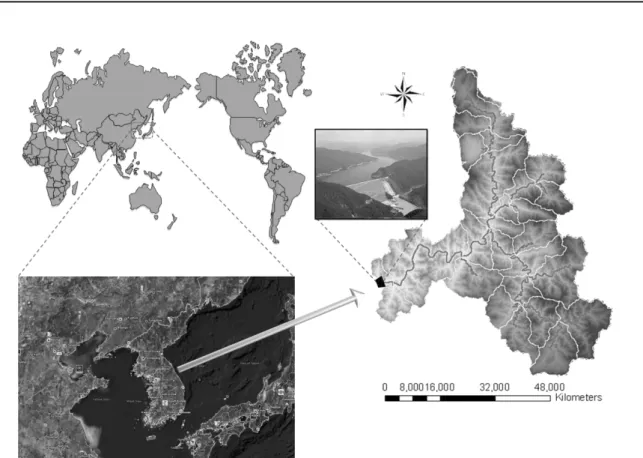
Soyanggang-dam watershed at Gangwon province, Korea was selected (Fig. 1) to demonstrate this study because long-term flow data with 12 precipitation gauging stations for this study watershed were available. The Soyanggang- dam watershed is located in typical monsoon climate area.
The coefficient of flow regime at this study watershed is huge due to greater precipitation during the summer.
2.3. Development of the Web-based flow clustering EI estimation system for SWAT Hydrologic Component Calibration
As stated earlier, the EI is affected by big numbers among a range of numbers. In this study, Web-based flow clustering EI estimation system was developed to evaluate SWAT estimated direct runoff and baseflow by calculating EI values after clustering direct runoff and baseflow data into 2 groups, respectively. For this, commonly used K- means clustering algorithm (MacQueen, 1967; Steinhaus, 1956) was utilized to develop Web-based flow clustering EI estimation system since it has been widely used in data clustering studies. In this study, the web interface was developed to provide this tool to SWAT users worldwide.
The Web-based flow clustering EI estimation system (http://www.envsys.co.kr/~fcei) (Fig. 2) was developed using the Perl/CGI and GNUPLOT to calculate the EI values of high-flow and low-flow groups of direct runoff and baseflow component of the SWAT estimation. As the Web-based flow clustering EI estimation system, developed in this study, is
Fig. 1. Location of the Soyanggang-dam watershed.
Fig. 2. Interface of the Web-based flow clustering EI estimation system.
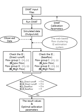
Fig. 3. Flow diagram of the Web-based flow clustering EI estimation system.
Web-based user-friendly module, most SWAT users could handle this EI estimation system with comparative ease.
The condensed processes of development of the Web- based flow clustering EI estimation system are given as follows. The EI error which is highly depending on big numbers among various data was analyzed; the overall K- means clustering algorithm was analyzed; data grouping interface was developed using the K-means clustering algo- rithm and Perl/CGI and GNUPLOT; the EI and K-means clustering algorithm were incorporated; calculation of the EI through tabular and graphical outputs are provided for the SWAT calibration.
The process of the calibration of the SWAT simulated flow using the Web-based flow clustering EI estimation system is given as follows (Fig. 3). First, run SWAT model with SWAT input parameter set; and then, obtain simulated data through the summary output file (output.std) in AVS- WATX; calculate the EI of simulated data and observed data using the Web-based flow clustering EI estimation system, developed in this study; check the EI values of flow group I and II of direct runoff as a positive value or not; check the EI values of flow groups I and II of base- flow as a positive value or not; if the EI values of 4 data groups (flow groups I and II of direct runoff and flow groups I and II of baseflow dataset) are all positive values, go to next step; else go back to first step until meet the
criteria (all positive EI values for 4 flow groups); the result value and optimal calibration parameters are come up with.
Flow group I is low value group and flow group II is high value group, clustered with K-means clustering algorithm;
low value and high value group hereafter called “flow group I and II” in this paper. Also, EI_L and EI_H are represen- tative EI value of flow group I and II in direct runoff and baseflow, respectively. Even though the calibration with the Web-based K-means clustering EI estimation module could get more accurate data than before, it spend lots of time in performing the SWAT calibration. Because it is calibration process for users to analyze EIs of direct runoff and base- flow in detail and examine one by one manually.
2.4. Direct runoff and baseflow separation using WHAT To evaluate the EI values for high and low flow groups of SWAT estimated direct runoff and baseflow values, measured flow data also should be first separated into direct runoff and baseflow components. Thus, direct runoff and baseflow were separated from measured flow data (year 2002 ~ 2005) of the Soyanggang-dam watershed, which were acquired from WAMIS (Water Resources Management Information System)(www.wamis.go.kr). The WHAT system provides three base flow separation modules; the local minimum method, parameter digital filter, and Eckhardt filter methods. The BFImax and filter parameter for the WHAT system were calculated through the BFImax analyzer in the WHAT system, and then daily direct runoff and baseflow were separated through the WHAT system.
2.5. Evaluation of the Web-based flow clustering EI esti- mation system
To demonstrate why the Web-based flow clustering EI estimation system is needed for accurate calibration of SWAT direct runoff and baseflow components, three case studies were carried out as follows. First, comparison of the SWAT manual calibration method vs. calibration with the Web-based flow clustering EI estimation system, and then the SWAT auto-calibration tool vs. calibration with the Web-based flow clustering EI estimation system was conducted. Third, EI values of total streamflow, direct run- off, and baseflow from the other SWAT application by Qi and Grunwald (2005) vs. using the Web-based flow clustering EI estimation system were compared.
The SWAT model input data (i.e., DEM, Land use, Soil, long-term weather data) (Table 1) were prepared for the study watershed to evaluate the Web-based flow clustering EI estimation system in calibrating SWAT hydrologic com- ponent. To simulate hydrology and nonpoint source loadings at steep sloping watersheds, SWAT ArcView GIS Patch II
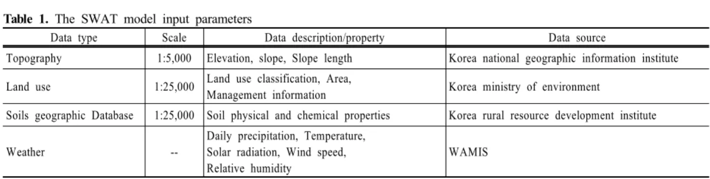
Table 1. The SWAT model input parameters
Data type Scale Data description/property Data source
Topography 1:5,000 Elevation, slope, Slope length Korea national geographic information institute Land use 1:25,000 Land use classification, Area,
Management information Korea ministry of environment
Soils geographic Database 1:25,000 Soil physical and chemical properties Korea rural resource development institute
Weather --
Daily precipitation, Temperature, Solar radiation, Wind speed, Relative humidity
WAMIS
(Kim et al., 2009; available at http://www.EnvSys.co.kr/
~swat)) was applied to minimize the effects of watershed delineation in SWAT estimated values. The SWAT ArcView GIS Patch II should be used if average slope of the water- shed is over 25% (Kim et al., 2009). The average slope of Soyanggang-dam watershed, study watershed in this study) is about 40.6%.
2.5.1. Comparison of the SWAT manual calibration vs. calibration with clustering EI estimation system
The SWAT manual calibration was carried out by com- paring total stream flow with measured streamflow until higher EI value is achieved. Also, for comparison of SWAT manual calibration with calibration using the Web- based flow clustering EI estimation system, the SWAT model direct runoff and baseflow were calibrated until all 4 positive EI values (EI_L and EI_H of direct runoff, and EI_L and EI_H of baseflow) of flow groups I and II of direct runoff and baseflow are achieved using the Web- based flow clustering EI estimation system. In the SWAT model, there are lots of parameters to be calibrated for best-fit between simulated and measured flow. In this study, several flow sensitive parameters (i.e., CN, ALPHA_
BF, GW_DELAY, GW_REVAP, and GWQMN) were adjusted manually for best-fit between simulated values and measured values. The calibrated parameter ranges were limited according to van Griensven et al. (2006) and Neitsch et al. (2005). Once the higher EI value from total stream flow comparison was achieved, the SWAT direct runoff and baseflow estimated with calibrated parameters using streamflow were compared with those calibrated using the Web-based flow clustering EI estimation system. In addition, EI_L and EI_H values of direct runoff and baseflow estimated with calibrated parameters were compared with those calibrated using the Web-based flow clustering EI estimation system.
2.5.2. SWAT auto-calibration tool vs. calibration with Web-based flow clustering EI estimation system
The AVSWAT has included the auto-calibration procedure that is used to obtain an optimal fit of process parameters.
The SWAT auto-calibration tool in AVSWAT was performed using statistical analysis to determine the reliability between the predicted and observed data. A parameter sensitivity analysis tool is embedded in SWAT to determine the rela- tive ranking of which parameters most affect the output variance due to input variability. It has objective functions which are aggregated to a single global criterion determined by optimal fit. The goodness-of-fit measure used was the EI (Green and Griensven, 2008). In this study, the EI values of total streamflow, direct runoff, and baseflow and EI values of flow group I (EI_L) and II (EI_H) clustered from direct runoff and baseflow were compared with using the SWAT auto-calibration tool and Web-based flow clustering EI estimation system.
2.5.3. Analysis of the EI values of Streamflow, direct runoff, and baseflow from the other SWAT application
Even though total streamflow, direct runoff, and baseflow has a good correlation between the simulated and observed data, flow group I and II could be bad fit between them.
So, the research results by Qi and Grunwald (2005) was selected and hydrological components from Qi and Grun- wald (2005)’s study was evaluated to investigate EI value of flow group I and II in direct runoff and baseflow using the Web-based flow clustering EI estimation system.
Qi and Grunwald (2005) evaluated the application of SWAT model for total streamflow, direct runoff, and base- flow occurring at 4 subwatersheds in the Sandusky watershed in USA. Exact numeric data for total stream flow, direct runoff, and baseflow were not provided in the research paper. Only graphs for total streamflow, direct runoff, and baseflow at 5 stations (i.e., Bucyrus, Fremont, Honey, Rock, and Tymochtee) were provided. In this study, result graphs of the study by Qi and Grunwald (2005) were interpreted to a numeric data to calculate the EI values using the Web-based flow clustering EI estimation system. These data were used to evaluate the EI values of flow group I (EI_L) and II (EI_H) of direct runoff and baseflow using the Web-based flow clustering EI estimation system.
3. Results and discussion
(a) Total streamflow
(b) Direct runoff and baseflow
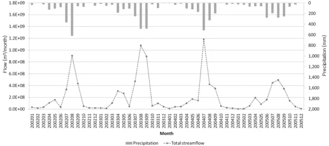
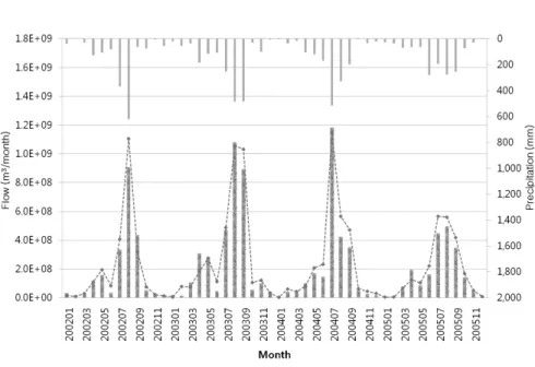
Fig. 4. Monthly total streamflow, direct runoff, and baseflow by the WHAT system.
3.1. Direct runoff and baseflow separation using the WHAT system
Daily flow data of the Soyanggang-dam watershed, mea- sured streamflow data, were separated using the WHAT system. Daily direct runoff and baseflow were divided through the WHAT system with the BFImax and filter parameters. The monthly average (year 2002 ~ 2005) total streamflow (measured data) were 210,717,540 m3/month, and direct runoff and baseflow (measured/filtered data) were 151,743,348 m3/month and 58,974,192 m3/month, respectively (Fig. 4).
According to the result graph as shown in Fig. 4 below, monthly average direct runoff and baseflow showed a ratio of 0.72 (72%) to 0.28 (28%) of total streamflow. In June 2005, direct runoff represented the highest number and monthly precipitation was about 280 mm while monthly
average precipitation was 133 mm during 2002 ~ 2005. At this time, direct runoff and baseflow were 147,618,720 m3/month (92%) and 13,068,000 m3/month (8%) respectively.
In Oct. 2004, baseflow appeared to be the highest and monthly precipitation was approximately 4 mm while monthly average precipitation was 133 mm during 2002 ~ 2005. Direct runoff and baseflow showed 11,105,856 m3/ month and 42,142,464 m3/month and their proportions were 21% and 79% individually at this moment.
3.2. Comparison of the SWAT manual calibration vs.
calibration with the Web-based flow clustering EI estimation system
Fig. 5(a) shows the comparison of simulated total stream- flow and measured total streamflow with the EI value of 0.95. The monthly average simulated total streamflow for
(a) Total streamflow
(b) Direct runoff and baseflow
Fig. 5. Monthly total streamflow, direct runoff, and baseflow w/ the SWAT manual calibration.
(m/c : The SWAT manual calibration)
year 2002 ~ 2005 was 232,928,714 m3/month, and direct runoff and baseflow were 225,528,610 m3/month and 7,400,104 m3/month separately. Daily direct runoff and baseflow were divided through the WHAT system with the BFImax and filter parameters. The monthly average (year 2002 ~ 2005) direct runoff and baseflow (measured/filtered data) were 151,743,348 m3/month and 58,974,192 m3/month, respectively (Fig. 5(b)). As shown in Fig. 5(a), SWAT users can judge that the SWAT calibration using only total stream flow was done reasonably well because of higher EI value of 0.95. However, simulated direct runoff values more or less overestimate measured direct runoff (EI value of 0.61) and simulated baseflow values were much lower than measured baseflow (EI value of -0.27). This result
indicates that calibration using total streamflow seemed to be impeccable but direct runoff and baseflow data would not.
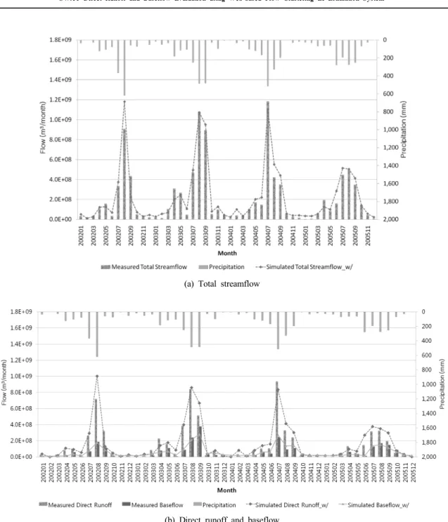
Fig. 6(a) shows the comparison of simulated total stream flow and measured total stream flow with EI value of 0.93 using Web-based flow clustering EI estimation system.
Here, flow group I and II of direct runoff and baseflow were calibrated using flow clustering EI estimation system until all positive EI_L and EI_H of direct runoff and baseflow were obtained. The EI value of 0.93 was achieved with the calibrated parameters for direct runoff and baseflow calibration using the flow clustering EI estimation system.
The monthly average simulated total streamflow for year 2002 ~ 2005 was 228,970,298 m3/month, and direct runoff
(a) Total streamflow
(b) Direct runoff and baseflow
Fig. 6. Monthly total streamflow, direct runoff, and baseflow w/ the Web-based flow clustering EI estimation system.
and baseflow were 168,824,829 m3/month and 60,145,469 m3/month separately. The monthly average (year 2002 ~ 2005) direct runoff and baseflow (measured/filtered data) were 151,743,348 m3/month and 58,974,192 m3/month, which were obtained from WHAT system (Fig. 6(b)).
While accuracy of total streamflow with the SWAT manual calibration is very similar to that with the Web- based flow clustering EI estimation system, direct runoff and baseflow between them look different (Fig. 5(b), 6(b)).
When comparing each hydrological component between with the SWAT manual calibration and Web-based flow clustering EI estimation system, direct runoff in Fig. 6(b) decreased by about 25% than that in Fig. 5(b) and base- flow in Fig. 6(b) increased by about 713% than that in
Fig. 5(b). This increased baseflow value has resulted in increased EI value (-0.27 to 0.92) of baseflow estimation.
With manual calibration, the EI value of 0.95 was achieved for total streamflow estimation. However, the EI_L and EI_H values of direct runoff and baseflow, esti- mated using the adjusted parameters through streamflow calibration process, were 0.63, -2.43, 0.63, -9.46 and -0.46, respectively (Table 2). With the Web-based flow clustering EI estimation system for more accurate calibration, the EI values of flow group I and II of direct runoff and baseflow in the Soyanggang-dam watershed were estimated. The EI value of total stream comparison was 0.93. The EI_L and EI_H values of direct runoff and baseflow, estimated using the adjusted parameters through streamflow calibration pro-
Table 2. Comparison of the EI values of the total streamflow, direct runoff, and baseflow I
Station Calibration for
total streamflow
Calibration for direct runoff
Calibration for baseflow
EI EI EI_L EI_H EI EI_L EI_H
Soyanggagng-dam_w/* 0.93 0.87 0.67 0.17 0.92 0.77 0.49
Soyanggang-dam_m/c** 0.95 0.61 0.63 -2.43 -0.27 -9.46 -0.46
*Soyanggang-dam_w/ : Calibration of total streamflow, direct runoff, and baseflow With the Web-based flow clustering EI estimation system
**Soyanggang-dam_m/c : Calibration of total streamflow, direct runoff, and baseflow With the SWAT manual calibration
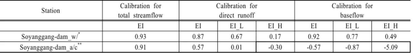
Table 3. Comparison of the EI values of the total streamflow, direct runoff, and baseflow II
Station Calibration for
total streamflow
Calibration for direct runoff
Calibration for baseflow
EI EI EI_L EI_H EI EI_L EI_H
Soyanggang-dam_w/* 0.93 0.87 0.67 0.17 0.92 0.77 0.49
Soyanggang-dam_a/c** 0.91 0.57 0.01 -0.30 -0.57 -0.87 -5.09
*Soyanggang-dam_w/ : Calibration of total streamflow, direct runoff, and baseflow With the Web-based flow clustering EI estimation system
**Soyanggang-dam_a/c : Calibration of total streamflow, direct runoff, and baseflow With the SWAT auto-calibration tool
cess, were 0.67, 0.17, 0.77, and 0.49, respectively (Table 2).
The EI values of total streamflow comparisons were very alike when manual calibration and calibration using the Web-based flow clustering EI estimation system were per- formed (EI values of 0.95 and 0.93, respectively). On the contrary, the EI_L and EI_H values of direct runoff and baseflow components were negative, except EI_L value of direct runoff when manual calibration was performed.
While, the EI_L and EI_H values of direct runoff and baseflow were all positive with the Web-based flow clus- tering EI estimation system. These results imply that SWAT hydrology component calibration using solely total stream- flow could result in errors of baseflow estimation, especially during low flow condition (Table 2).
3.3. The SWAT auto-calibration tool vs. calibration with the Web-based flow clustering EI estimation system The SWAT auto-calibration tool was utilized to calibrate the hydrology component of SWAT. The EI value of total streamflow was 0.91, which is somewhat similar to that obtained from manual calibration and calibration using flow clustering EI estimation system (0.95 and 0.93, respec- tively). However, even with the auto-calibration tool, embe- dded in the SWAT, the EI_L and EI_H values of direct runoff and baseflow were 0.01, -0.30, -0.87, and -5.09 (Table 3). As shown in this study, the higher EI value from total streamflow comparison does not guarantee higher accuracies in estimated direct runoff and baseflow estimation.
3.4. Analysis of EI values of Streamflow, direct runoff, and baseflow from the other SWAT application
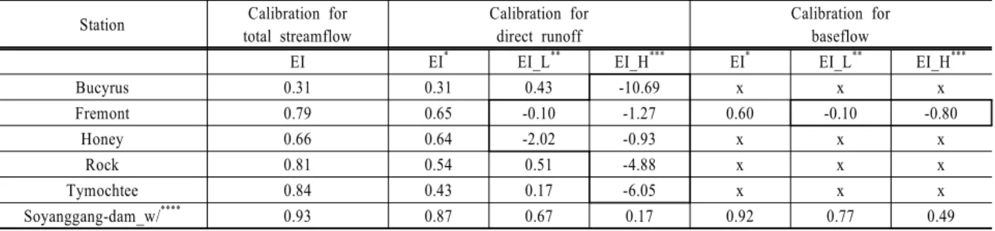
While the EI values of the total streamflow, direct runoff, and baseflow in the research result by Qi, and Grunwald (2005) were positive values, most EI values (EI_L and EI_H) of direct runoff and baseflow were negative values after clustering direct runoff and baseflow into each flow group I (EI_L) and II (EI_H) using the Web-based flow clustering EI estimation system as shown in Table 4.
In contrast to the EI values in the study by Qi and Grunwald (2005), which were most negative values (-10.69
~ -0.10), the EI values of each flow group I (EI_L) and II (EI_H) in direct runoff and baseflow in the Soyanggang- dam watershed were all positive values. EI_L and EI_H of direct runoff and baseflow showed 0.67, 0.17, 0.77, and 0.49 respectively. Thus, SWAT model should be calibrated for various flow regime (flow group I and II of direct runoff and baseflow), not only using streamflow, or either direct runoff and baseflow.
4. Conclusion
When hydrological component has been calibrated and validated by various SWAT users, most SWAT users have evaluated accuracy of hydrological component through only total streamflow using the EI. As the EI was affected sensitively by big numbers among a range of data, hydrologic modeling had problems for accurate estimation in the dry (low flow) season. Thus, many researches have been conducted to develop better statistic than the EI to remove the effects of big numbers in SWAT estimation.
Thus, in this study the Web-based flow clustering EI estimation system was developed and applied in the
Table 4. Comparison of the EI values of the total streamflow, direct runoff, and baseflow III (Qi and Grunwald, 2005) Station Calibration for
total streamflow
Calibration for direct runoff
Calibration for baseflow
EI EI* EI_L** EI_H*** EI* EI_L** EI_H***
Bucyrus 0.31 0.31 0.43 -10.69 x x x
Fremont 0.79 0.65 -0.10 -1.27 0.60 -0.10 -0.80
Honey 0.66 0.64 -2.02 -0.93 x x x
Rock 0.81 0.54 0.51 -4.88 x x x
Tymochtee 0.84 0.43 0.17 -6.05 x x x
Soyanggang-dam_w/**** 0.93 0.87 0.67 0.17 0.92 0.77 0.49
*EI : Nash and Sutcliffe effective index for total data set;
**EI_L : Nash and Sutcliffe effective index for low value group data set (flow group I);
***EI_H : Nash and Sutcliffe effective index for high value group data set (flow group II);
****Soyanggang-dam_w/ : Calibration of total streamflow, direct runoff, and baseflow With the Web-based flow clustering EI estimation system x : No data
Soyanggang-dam watershed. The EIs of each flow group I and II, four EIs, clustered from direct runoff and baseflow was calculated and it showed four EI values (i.e., EI_L and EI_H of direct runoff were 0.67, 0.17 and EI_L and EI_H of baseflow were 0.77, 0.49) were bigger than zero.
With all positive EI values (EI_L and EI_H of direct runoff and baseflow components), higher EI values for direct runoff comparison (EI of 0.87) and baseflow (EI of 0.92) were obtained. In addition, the EI value of 0.93 was achieved for total streamflow comparison.
With the SWAT manual calibration, even though the EI of total streamflow was very high (0.95), the EIs of each flow group I and II, four EI values were low (i.e., EI_L and EI_H of direct runoff were 0.63, -2.43 and EI_L and EI_H of baseflow were -9.46, -0.46). Also with SWAT auto-calibration tool, the EI of total streamflow was high (0.91). However, the EIs of each flow group I and II, four EI values were lower than those with manual calibration (i.e., EI_L and EI_H of direct runoff were 0.01, -2.30 and EI_L and EI_H of baseflow were -0.87, -5.09).
Therefore, calibration and validation of hydrological component in the SWAT should be performed using the Web-based flow clustering EI estimation system developed in this study for more accurate hydrologic component estimation, especially during low flow season, or baseflow.
요 약
유역 단위 수문 및 수질 평가 모형인 SWAT 모형을 이 용한 유역 내 정확한 수문과 비점오염원 거동을 평가하기 위해서는 유역 적용에 앞서 모형의 정확성 평가가 우선시 되어야 한다. SWAT 모형의 수문 보정및 검정 시, Nash-Sutcliffe의 효율계수(EI)가 널리 사용되고 있다. 그러 나 이러한 EI 값은 비교되어지는 값들의 범위 중 큰 값 즉, 수문 분석에 있어 고유량에 대해 민감하게 영향을 받 는 것으로 알려져 있다. 그리하여 본 연구에서는 보다 정
확한 수문 분석을 위해 K-means 군집화 알고리즘을 이용 한 웹기반의 EI 평가시스템을 개발하였고, 이를 SWAT 모 형의 수문 평가에 적용하였다. 본 연구의 결과 전체 유량 의 EI 값은 높았지만, 수문성분에 따른 EI 값은 높지 않았 다. SWAT 모형의 수문 보정 및 검정에 널리 활용되고 있 는 SWAT auto-calibration tool은 전체 유량에 대해서는 높 은 EI 값을 산정하는 것으로 보이지만, 직접유출과 기저유 출 각각에 대한 유량 그룹 I 과 II 에 대해서는 대부분 음수 (-)의 EI 값을 보였다. 그리하여 본 연구 결과를 통해 SWAT 모형의 수문성분 평가에 있어 보다 정확한 평가를 위해서는 직접유출과 기저유출에 대한 각각의 유량 그룹에 대해 양수(+)의 EI 값이 산정되도록 모형 보정 및 검정의 수행 필요할 것으로 사료된다.
Acknowledgment
We express gratitude to a Grant (code: 2-2-3) from the Sustainable Water Resources Research Center of “the 21st Century Frontier Research Program”, and Korea Ministry of Environment which supports this project as “the GAIA Project”, and also would like to thank the editor and anony- mous reviewers for the valuable comments and suggestions, which greatly enhanced the quality of this manuscript.
References
Arnold, J. G., Srinivasan, R., Muttiah, R. S., and Williams, J.
R. (1998). Large area hydrologic modeling and assessment:
part I: model development. Journal of American Water Resources Association, 34(1), pp. 73-89.
Bicknell, B. R., Imhoff, J. C., Donigian, A. S., and Johanson, R. C. (1997). Hydrological Simulation Program-FOTRAN (HSPF). User’s Manual for release 11(EPA-600/R-97/080), United States Environmental Protection Agency, Athens, GA.
Cao, F., Liang, J., and Jiang, G. (2009). An initialization method for the Web-based K-means algorithm using neighborhood model. Computers and Mathematics with Applications, 58,
pp. 474-483.
Cho, J., Park, S., and Lm, S. (2008). Evaluation of Agricultural Nonpoint Source (AGNPS) model for small watersheds in Korea applying irregular cell delineation. Agricultural Water Management, 95(4), pp. 400-408.
Chow, V. T., Maidment, D. R., and Mays, L. W. (1988).
Applied Hydrology, McGraw-Hill, New York.
Cryer, S. A. and Havens, P. L. (1999). Regional sensitivity analysis using a fractional factorial method for the USDA model GLEAMS. Environmental Modeling and Software, 14(6), pp. 613-624.
Green, C. H. and Van Griensven, A. (2008). Autocalibration in hydrologic modeling: Using SWAT 2005 in small-scale watersheds. Environmental Modelling & Software, 23, pp.
422-434.
Gupta, H. V., Sorooshian, S., and Yapo, P. O. (1999). Status of automatic calibration for hydrologic models: comparison with multilevel except calibration. Journal of Hydrologic Engineering, 4(2), pp. 135-143.
Kim, J., Park, Y., Yoo, D., Kim, N., Engel, B. A., Kim, S., Kim, K., and Lim, K. J. (2009). Development of a SWAT patch for better estimation of sediment yield in steep sloping watersheds. Journal of the American Water Resources Association, 45(4), pp. 963-972.
Lim, K. J., Engel, B. A., Tang, Z., Choi, J., Kim, K., Muthu- krishnan, S., and Tripathy, D. (2005). Automated Web GIS-based Hydrograph Analysis Tool, WHAT. Journal of the American Water Recourse Association, 41(6), pp. 1407-1416.
Lloyd, S. P. (1957). Least square quantization in PCM. Bell Telephone Laboratories Paper. Published in journal much later: S. P. Lloyd (1982). Least squares quantization in PCM. IEEE Transactions on Information Theory, 28(2). pp.
129-137.
MacQueen, J. B. (1967). Some Methods for classification and Analysis of Multivariate Observations. Proceedings of 5th Berkeley Symposium on Mathematical Statistics and Proba- bility, University of California Press, 1, pp. 281-297.
McCuen, R. H., Knight, Z., and Cutter, A. G. (2006).
Evaluation of the Nash-Sutcliffe Efficiency Index, Journal of Hydrologic Engineering, 11(6), p. 597.
Nash, J. E. and Sutcliffe, J. V. (1970). River flow forecasting through conceptual models. Part 1: A discussion of prin- ciples. Journal of Hydrology, 10(3), pp. 282-290.
Neitsch, S. L., Arnold, J. G., Kiniry, J. R., Srinivasan, R., and Williams, J. R. (2005). Soil and Water Assessment Tool (SWAT) Users Manual. BRC(02-06), Blackland Research Center, Texas Agricultural Experiment Station, Temple, Texas.
Qi, C. and Grunwald, S. (2005). GIS-Based hydrologic mode- ling in the Sandusky watershed using swat. American Society of Agricultural Engineers, 48(1), pp. 169-180.
Rossman, L. A. (2009). Storm Water Management Model User’s Manual Version 5.0. EPA/600/R-05/040, National Risk Management Research Laboratory, United States Environ- mental Protection Agency, Cincinnati, Ohio.
Steinhaus, H. (1956). Sur la division des corps matériels en parties, Bull. Acad. Polon. Sci., 1, pp. 801-804.
Van Grienven, A., Francos, A., and Bauwens, W. (2002).
Sensitivity analysis and auto-calibration of an integral dynamic model for river water quality. Water Science and Technology, 45(9), pp. 325-332.
Van Griensven, A., Meixner, T., Grunwald, S., Bishop, T., Di luzio, M., and Srinivasan, R. (2006). A global sensitivity analysis tool for the parameters of multi-variable catchment models. Journal Hydrology, 324, pp. 10-23.
Walling, D. E., He, Q., and Whelan, P. A. (2003). Using 137Cs Measurements to validate the application of the AGNPS and ANSWERS erosion and sediment yield modles in two small Devon Catchments. Soil and Tillage Research, 69(1-2), pp. 27-43.
Zhou, H., and Liu, Y. (2008). Accurate integration of multi- view range image using k-means clustering. The Journal of the Pattern Recognition Society, 41(1), pp. 152-175.