Key block analysis method for
observational design and construction method in tunnels
Jae-Yun Hwang
1*
터널의 정보화 설계시공을 위한 키블럭 해석기법
황재윤
Abstract Recently, the observational design and construction method in tunnels has been becoming important. Rock masses include various discontinuities such as joints, faults, fractures, bedding planes, and, cracks. The behavior of tunnels in hard rocks, therefore, is generally controlled by various discontinuities. In this study, a new key block analysis method for observational design and construction method in tunnels is proposed, and then applied to the actual tunnel with a super-large cross-section. The proposed analysis method considers finite persistence of discontinuities. The new analysis method can handle concave and convex shaped blocks. To demonstrate the applicability of this key block analysis method for observational design and construction method in tunnels, the analysis results are examined and compared with those of the conventional method.
Keywords: Key block analysis method, observation design and construction method, persistence, tunnel
요 지 최근 터널의 정보화 설계시공이 중요시 되어지고 있다. 암반에는 절리, 단층, 균열, 층리, 단열 등의 불연속면이 많이 포함되어 있다. 따라서, 암반 불연속면이 터널의 거동을 좌우하고 있다. 본 연구에서는 터널의 정보화 설계시공을 위한 키블럭 해석기법을 제안하고, 초대단면 터널현장에 적용했다. 제안한 해석기법은 불연속면의 연속성을 고려하여, 블록의 형상에 관계없이 모든 형상의 블록이 인식 가능하여 복잡한 굴착면에 적용가능하다. 터널현장에서의 해석결과를 비교 검토 하여, 본 연구에서 개발한 터널의 정보화 설계시공을 위한 키블럭 해석기법의 타당성과 적용성에 대한 검증을 하였다.
주요어: 키블럭 해석기법, 정보화 설계시공, 연속성, 터널
1. Introduction
The properties of rock masses are very important factors in the design and construction of tunnels. Rock masses in nature contain a great variety of discontinuities such as faults, joints, fractures, bedding planes, seams, cracks, schistosities, fissures and cleavages. The behavior of civil structures in hard rocks, therefore, is mainly controlled by numerous discontinuities (Ohnishi, 2002;
Hwang, 2003; Hwang et al., 2004). The tunnel support design has been mostly empirical. The typical support design pattern is based on the rock/soil types, or based on the rock mass classification. However, both stress and rock structure induced failures should be considered in the design of rock support for tunnel design.
As for the assessment of the rock structure induced failures, the so-called block theory was suggested by Goodman and Shi (1985). Excavations in discontinuous rock masses are frequently affected by key blocks, which are critical blocks of rock bounded by discontinuities and excavation surfaces. Block theory is a geometrically based on set of techniques that determine where dangerous blocks may exist in a rock mass intersecting by variously oriented discontinuities in three dimensions. Block theory is a quite useful method to determine the stability of rock blocks that were created by the intersection of discontinuities and the excavated surfaces. However, the block theory is based on some assumptions which limit its usefulness. In block theory, joint surfaces are assumed to extend entirely through the volume of interest; that is, no discontinuities will terminate within the region of a key block (Ohnishi et al., 1985).
한국터널공학회논문집 2010년 5월 제12권 제3호, pp. 275-283
1
종신회원, 부산광역시의회 정책연구실 선임연구위원, 공학박사
*교신저자: 황재윤 (E-mail: [email protected])
학술논문
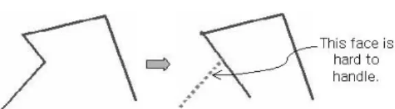
infinite persistent discontinuities, and does not consider the effects of finite discontinuity persistence, therefore cannot deal with a complex concave shaped block (Fig. 1). The rock block should be divided into convex sub-blocks. In practice, it is necessary to consider the persistence of finite discontinuities to attempt applying the block theory to successive excavations.
In this study, a new key block analysis method for observational design and construction method in tunnels is proposed, and then applied to the actual large tunnel. Three-dimensional rock block identification with consideration of the persistence of discontinuities is performed by using discontinuity disk model. The removability and stability analyses of rock blocks formed by the rock block identification method are performed. The new analysis method for observational design and construction method in tunnels can handle concave and convex shaped blocks.
2. 3D Discontinuous Rock Mass Modeling 2.1 Discontinuity disk model
To build a 3D model considering finite discontinuity persistence, the problem concerned with geometric shape and spatial extent of discontinuities must be addressed.
Through the analysis of trace data and examination of discontinuity surfaces, several studies (Warburton, 1980; Long and Billaux, 1987; Pollard and Aydin, 1988; Priest, 1993; Ohnishi et al., 1994) have demonstrated that discontinuities are likely to be roughly elliptical or circular.
The fundamental basis of the discontinuity disk model is the assumption of circular discontinuity
shapes (Ohnishi et al., 1994; Mardia, 1972; Pahl, 1981; Dershowitz, 1984; Kulatilake et al., 1993; Zhang and Einstein, 2000) as shown in Fig. 2.
The size of circular discontinuities is defined completely by a single parameter, the discontinuity radius. Discontinuity radius may be defined deterministically, as a constant for all discontinuities, or stochastically by a distribution of radii. The best and most widely adopted sampling strategy for determining discontinuity size is based on the measurement of the lengths of the traces produced where the discontinuities intersect a planar face (Priest, 1993). The probability distribution of discontinuity diameters may be inferred from the distribution of the trace length, which can be measured through excavation surfaces or natural outcrops. However, the direct estimation of trace lengths is often influenced by varied biases, and the distribution inferred from trace length involves integration that can only be evaluated numerically, and this also becomes a barrier when building a statistical model with Monte Carlo simulation. To overcome these problems, the stochastic discontinuity system modeling process of this developed program first assumes that discontinuity diameter and trace length have the same distribution function (e.g., lognormal or exponential distribution), then determines the mean and standard deviation of discontinuity diameters through model calibration. Discontinuity location may also be defined by a deterministic pattern or a stochastic process. The most frequently used model to define the spatial location of stochastic discontinuities is the
Fig. 2. Discontinuity disk model.
Key block analysis method for observational design and construction method in tunnels
Poisson model. In the discontinuity system modeling process of this developed program, the spatial location of stochastic discontinuities was assumed to follow the Poisson model. As a result of the discontinuity location, shape and size process of the discontinuity disk model, discontinuities terminate in rock and intersect each other.
2.2 Analysis region modeling
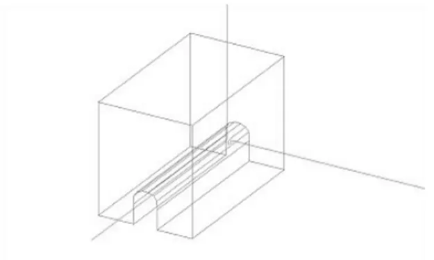
The model region of this study is a closed domain with a certain number of faces. Model region may be of any shape closed by polygons. The excavation faces may be convex or concave polygonal faces with or without interior holes. All excavation faces should form a closed domain of target rock mass for the analysis; if they do not form a closed domain, some fabricated faces, such as boundary faces, should be added. A curve face should be approximated by a number of polygonal faces. Fig. 3 shows an example of the analysis region modeling for an underground cavern.
3. Identification of 2D Loop
In a discontinuity system, not all discontinuities (which may be deterministic or generated by stochastic simulation) are connected; some discontinuities do not intersect
with other discontinuities, and some discontinuities intersect with very few discontinuities (Yu, 2000).
Before the rock block identification stage, unconnected discontinuities should be identified and eliminated. In order to reduce computational requirement, some discontinuities may be considered unconnected and eliminated because of their small sizes.
A discontinuity is referred to as connected only when it plays a part in block formation (i.e., it forms a surface of some block). A connected discontinuity must feature the two following characteristics: (1) it is connected to at least 3 discontinuities including excavation faces, (2) within the planar disk of the considered discontinuity, the intersections between the considered discontinuity and other connected discontinuities or excavation faces must form at least one connected loop. Fig. 4 shows some cases of connected and unconnected discontinuities.
By checking every discontinuity against the two characteristics mentioned above, all unconnected discontinuities can be identified and eliminated. It should be noted that this is an iteration procedure.
Some discontinuities, which look connected, may be identified to be unconnected after unconnected discontinuities are eliminated.
4. Identification of 3D Loop
A whole discontinuity does not form a surface of block. Therefore, after the elimination of unconnected
Fig. 3. An example of analysis region modeling for an underground cavern.
(a) Unconnected (b) Connected
Fig. 4. Cases of unconnected discontinuity and connected
discontinuity.
A face in 3D closed region forms when other discontinuities cut the region. 2D line loop should be established at the surfaces of the three-dimensional region. When this criterion is satisfied at all faces, one or more blocks are formed.
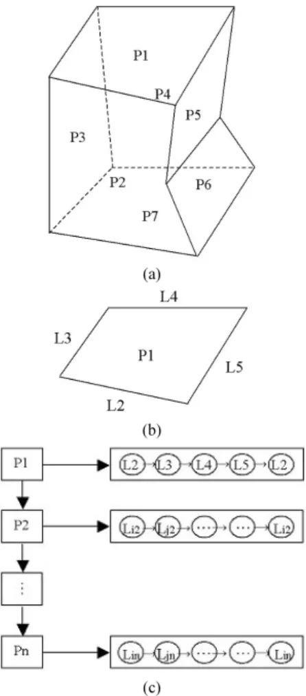
The algorithm of the 3D loop is demonstrated graphically by an example in Fig. 5. One individual 2D loop may be represented by its boundary nodes arranged in clockwise direction or counter-clockwise direction. The 3D loop may also be represented by its boundary 2D loops arranged in clockwise direction
Consequently, a block is represented by a number of 3D loops; a 3D loop is represented by a number of 2D loops; a 2D loop is represented by the nodes on its boundaries; and a node is described by 3D coordinates. Naturally, all the above identification processes will be accomplished automatically by computer.
5. Finalization of Block Shape and Volume
The volume of blocks will be determined by a simplex integration method. Simplex integration method is an accurate solution on n-dimensional domains with any shape. Simplex integration is based on the topology (Shi, 2001). The simplex has the most simple shape in 0, 1, 2, 3, …, n dimensional space as shown in Fig.
6. Different from the ordinary integration, the simplex integration has only the simplex as the integral domain.
The simplex also has positive and negative orientations.
The positive and negative orientations are defined as positive and negative volumes respectively.
The coordinates of the vertices V
0, V
1, V
2, V
3on any 3D simplex are supposed as (x
0, y
0, z
0), (x
1, y
1, z
1), (x
2, y
2, z
2) and (x
3, y
3, z
3) respectively. Therefore, the volume of the 3D simplex V
0V
1V
2V
3is
1 1 1 1
! 3 1
3 3 3
2 2 2
1 1 1
0 0 0
z y x
z y x
z y x
z y x
V = (1)
(a)
(b)
(c)
Fig. 5. 3D loop. Fig. 6. 0-, 1-, 2-, 3-Dimensional simplex
Key block analysis method for observational design and construction method in tunnels
The volume of simplex V
1V
0V
2V
3is the negative volume of simplex V
0V
1V
2V
3.
The integration formulas on the domain of 3D simplex V
0V
1V
2V
3(Fig. 6) with non-zero volume can be represented as follows (Shi, 2001). Supposing (x
0, y
0, z
0), (x
1, y
1, z
1), (x
2, y
2, z
2) and (x
3, y
3, z
3) are the coordinates of the vertices V
0, V
1, V
2, and V
3respectively.
Set
3 3 3
2 2 2
1 1 1
0 0 0
1 1 1 1
z y x
z y x
z y x
z y x
J = (2)
The formulas for the 3D simplex integrations, that the integrands are the degree of 0, 1 and 2, can be represented as follows.
J J
dxdydz J
sign z y x
D
vvvvv v v v
6 1 )!
3 0 (
! 0 ) ( ) , , (
1
01233 2 1 0
+ =
=
= ∫
∫ (3)
) 24 (
1
) )! (
1 3 (
! 1 ) ( ) , , (
3 2 1 0
3 2 1 0 3 2 1 0 3
2 1 0
x x x x J
x x x x J
xdxdydz J
sign z y x
xD
vvvvv v v v
+ + +
=
+ + + +
=
= ∫
∫
(4)
) 24 (
1 ) ( ) , , (
3 2 1 0
3 2 1 0 3
2 1 0
y y y y J
ydxdydz J
sign z y x
yD
vvvvv v v v
+ + +
=
= ∫
∫ (5)
) 24 (
1 ) ( ) , , (
3 2 1 0
3 2 1 0 3
2 1 0
z z z z J
zdxdydz J
sign z y x
zD
vvvvv v v v
+ + +
=
= ∫
∫ (6)
) 2 2 2 2 ( 120
1 ) ( ) , , (
3 3 2 3 1 3 0 3
3 2 2 2 1 2 0 2
3 1 2 1 1 1 0 1
3 0 2 0 1 0 0 0
2 2
3 2 1 0 3
2 1 0
x x x x x x x x
x x x x x x x x
x x x x x x x x
x x x x x x x x J
dxdydz x J sign z y x D
x
vvvvv v v v
+ + + +
+ + + +
+ + + +
+ + +
=
= ∫
∫
(7)
) 2 2 2 2 ( 120
1 ) ( ) , , (
3 3 2 3 1 3 0 3
3 2 2 2 1 2 0 2
3 1 2 1 1 1 0 1
3 0 2 0 1 0 0 0
2 2
3 2 1 0 3
2 1 0
y y y y y y y y
y y y y y y y y
y y y y y y y y
y y y y y y y y J
dxdydz y J sign z y x D
y
vvvvv v v v
+ + + +
+ + + +
+ + + +
+ + +
=
= ∫
∫
(8)
) 2 2 2 2 ( 120
1 ) ( ) , , (
3 3 2 3 1 3 0 3
3 2 2 2 1 2 0 2
3 1 2 1 1 1 0 1
3 0 2 0 1 0 0 0
2 2
3 2 1 0 3
2 1 0
z z z z z z z z
z z z z z z z z
z z z z z z z z
z z z z z z z z J
dxdydz z J sign z y x D
z
vvvvv v v v
+ + + +
+ + + +
+ + + +
+ + +
=
= ∫
∫
(9)
) 2 2 2 2 ( 120
1 ) ( ) , , (
3 3 2 3 1 3 0 3
3 2 2 2 1 2 0 2
3 1 2 1 1 1 0 1
3 0 2 0 1 0 0 0
3 2 1 0 3
2 1 0
y x y x y x y x
y x y x y x y x
y x y x y x y x
y x y x y x y x J
xydxdydz J
sign z y x
xyD
vvvvv v v v
+ + + +
+ + + +
+ + + +
+ + +
=
= ∫
∫
(10)
) 2 2 2 2 ( 120
1 ) ( ) , , (
3 3 2 3 1 3 0 3
3 2 2 2 1 2 0 2
3 1 2 1 1 1 0 1
3 0 2 0 1 0 0 0
3 2 1 0 3
2 1 0
z x z x z x z x
z x z x z x z x
z x z x z x z x
z x z x z x z x J
xzdxdydz J
sign z y x
xzD
vvvvv v v v
+ + + +
+ + + +
+ + + +
+ + +
=
= ∫
∫
(11)
) 2 2 2 2 ( 120
1 ) ( ) , , (
3 3 2 3 1 3 0 3
3 2 2 2 1 2 0 2
3 1 2 1 1 1 0 1
3 0 2 0 1 0 0 0
3 2 1 0 3
2 1 0
z y z y z y z y
z y z y z y z y
z y z y z y z y
z y z y z y z y J
yzdxdydz J
sign z y x
yzD
vvvvv v v v