Study of Hybrid Optimization Technique for Grain Optimum Design

(1)

Received: March 17, 2017 Revised: September 25, 2017 Accepted: September 29, 2017

780

http://ijass.org pISSN: 2093-274x eISSN: 2093-2480

Paper

Int’l J. of Aeronautical & Space Sci. 18(4), 780–787 (2017) DOI: http://dx.doi.org/10.5139/IJASS.2017.18.4.780

Study of Hybrid Optimization Technique for Grain Optimum Design

Seok-Hwan Oh, Yong-Chan Kim, Seung-Won Cha*, and Tae-Seong Roh**

Department of Aerospace Engineering, Inha University, Incheon 22212, Republic of Korea

Abstract

The propellant grain configuration is a design variable that determines the shape and performance of a solid rocket motor. Grain configuration variables have complicated effects on the motor performance; so the global optimization problem has to be solved in order to design the configuration variables. The grain performance has been analyzed by means of the grain burn-back and internal ballistic analysis, and the optimization technique searches for the configuration variables that satisfy the requirements. The deterministic and stochastic optimization techniques have been applied for the grain optimization, but the results are imperfect. In this study, the optimization design of the configuration variables has been performed using the hybrid optimization technique, which combines those two techniques. As a result, the hybrid optimization technique has proved to be efficient for the grain optimization design.

Key words: Solid rocket motor, Propellant grain, Optimal design, Hybrid optimization technique

Nomenclature

Ab : Burning surface area Ap : Port area

L : Grain length

mg : Rate of mass generation mn : Mass though the nozzle M : Mass stored in the chamber ρp : Propellant density

rb : Burning ratio α : Propellant coefficient n : Burning-rate pressure index Pc : Combustion-chamber pressure At : Nozzle throat area

C* : Characteristic speed of the propellant t : Time

v : Chamber volume

Tc : Combustion-chamber gas temperature g0 : Gravitational acceleration at sea level Cf : Thrust coefficient

F : Thrust

Obj : Objective function

Fobjective : Target thrust profile

Fcalculation : Internal ballistic calculation result j : Iteration

Fobjective_avg : Average target thrust profile

1. Introduction

The solid rocket motor (SRM) is made up of grain, ignitor, motor case, and nozzle. The outer configuration of the grain influences the motor size, and the inner configuration determines the SRM performance; so the grain design is very important for the SRM total design. In the SRM design process, the thrust profiles are given variously according to the mission requirements, which the grain redesign needs to consider [1,2]. The grain can be designed using the configuration variables. The thrust profile is a function of the configuration variables, and each configuration variable has a complicated effect on it. Finding the configuration variables is a nonlinear global optimization problem with many local solutions [3].

Optimization techniques can be applied to appropriately obtain these configuration variables. A grain-configuration optimization code has been developed by linking grain

. .

This is an Open Access article distributed under the terms of the Creative Com-mons Attribution Non-Commercial License (http://creativecomCom-mons.org/licenses/by- (http://creativecommons.org/licenses/by-nc/3.0/) which permits unrestricted non-commercial use, distribution, and reproduc-tion in any medium, provided the original work is properly cited.

* Ph. D Student

** Professor, Corresponding author: [email protected]

(2)

781

Seok-Hwan Oh Study of Hybrid Optimization Technique for Grain Optimum Design

http://ijass.org burn-back analysis [4], internal ballistic analysis [5], and

an optimization process in order to confirm whether the optimization technique is useful for designing the configuration variables. Optimum configuration design has been performed by applying deterministic or stochastic techniques. However, configuration design has sometimes failed because of the disadvantages of each optimization technique.

The deterministic method is excellent for searching for the optimum solution, but for optimizing a large area, the computation time may increase and fall into the local solution [6]. The stochastic method can perform most of the optimization design, but its search performance near the optimum solution is low [7]. In order to carry out the grain configuration design, the optimization technique suitable for configuration variables should be searched for and applied.

In this study, a hybrid optimization technique has been developed by using the merits of existing optimization techniques, offsetting their shortcomings, and applying them to optimize the configuration variables. It has been confirmed that the developed hybrid optimization technique is useful for configuration variable design.

2. Optimal design of Solid rocket motor

2.1 Optimal design process of grain configuration

In order to optimize the grain design, the grain burn-back analysis module, the internal ballistic analysis module, and the optimization module should be linked, as shown in Fig. 1 [5]. The grain burn-back analysis module analyzes the change in grain configuration during combustion, while the internal ballistic analysis module calculates the performance of the SRM [8]. If the performance does not meet the requirements, the configuration variables are redesigned by use of the optimization module [9].

2.2 Grain burn-back analysis module

The grain configuration, such as the burning surface area and the port area, changes during the combustion process. Since the configuration change affects the performance, such as thrust, it is

necessary to analyze the combustion configuration by using the grain burn-back analysis. In this study, we developed the grain burn-back analysis module using a geometric interpretation of the propellant configuration to calculate the burning surface area and the port area as a function of configuration variables [10]. The burning surface area and the port area are used for the internal ballistic analysis, and the new grain configuration is analyzed by applying the results calculated in the internal ballistic analysis to the grain burn-back analysis.

The slot and star configurations and variables are shown in Fig. 2 and Table 1. The slot grain has five configuration variables (N, R0, Ri, w, f ) and the star grain has six configuration variables (N, R0, Ri, w, f, ε). The equations for calculating the burning surface area and port area are different, depending on the set of configuration variables. For example, the slot configuration in Fig. 2 can be calculated by using Eqs. 1 and 2, and when the condition is changed, as when the entire web is burned, the grain burn-back analysis is conducted by changing to the corresponding Eqs. 3 and 4 [4].

4

calculated by using Eqs. 1 and 2, and when the condition is changed, as when the entire web is burned, the grain burn-back analysis is conducted by changing to the corresponding Eqs. 3 and 4 [4].

Fig. 2. Slot and star grain configuration and variables Table 1. Grain configuration variables

N Number of slot/star branch

0 R External radius(mm) i R Internal radius(mm) w Web thickness(mm) f Fillet radius(mm)  Angle coefficient 2 2 0 2 2  _{ }       _ _{ }      _  __       b i i a A NL f R w f R f R N , (1) 2 2 2 2 2 2 0 1 ₂ 1 2 2 2  _{ }       _  _  _   _     __       p i a i i A NL f R _N f R f f R w f R f , (2) 2 2 2       _     _  __     b b p i i a A NL f R R f R N , (3)









2 2 2 2 2 2 0 0 0 2 2 sin 2  _{ }      _  _ _ _ _     _ _      _ _   __ _{ } _ _ _ __ _  _ _ _ _   i a p i p c b c f R f R R f N A NL R w f R f R (4)









2 2 2 0 1 1 1 0

sin , cos , sin sin

2 2 2           _ _ _  _ _ _  _ _ _ __      _ _          _  _      p a b c b i p R R y f y f y f R y R y f R . , (1) 4

0 R External radius(mm) i R Internal radius(mm) w Web thickness(mm) f Fillet radius(mm)  Angle coefficient 2 2 0 2 2  _{ }       _ _{ }      _  __       b i i a A NL f R w f R f R _N , (1) 2 2 2 2 2 2 0 1 ₂ 1 2 2 2  _{ }       _  _  _   _     __       p i a i i A NL f R f R f f R w f R f N , (2) 2 2 2       _     _  __     b b p i i a A NL f R R f R _N , (3)









2 2 2 2 2 2 0 0 0 2 2 sin 2  _{ }      _  _ _ _ _     _ _      _ _   __ _{ } _ _ _ __ _  _ _ _ _   i a p i p c b c f R _N f R R f A NL R w f R f R (4)









2 2 2 0 1 1 1 0

sin , cos , sin sin

2 2 2                            _ _          _  _      p a b c b i p R R y f y f y f R y R y f R . 4

0 R External radius(mm) i R Internal radius(mm) w Web thickness(mm) f Fillet radius(mm)  Angle coefficient 2 2 0 2 2  _{ }       _ _{ }      _  __       b i i a A NL f R w f R f R _N , (1) 2 2 2 2 2 2 0 1 ₂ 1 2 2 2  _{ }       _  _  _   _     __       p i a i i A NL f R f R f f R w f R f N , (2) 2 2 2       _     _  __     b b p i i a A NL f R R f R N , (3)

















2 2 2 0 1 1 1 0

sin , cos , sin sin

2 2 2                         _ _     _ _  __       _  _      p a b c b i p R R y f y f y f R y R y f R . , (2) 3

not meet the requirements, the configuration variables are redesigned by use of the optimization module [9].

Fig. 1 Grain optimal design process

2.2 Grain burn-back analysis module

The grain configuration, such as the burning surface area and the port area, changes during the combustion process. Since the configuration change affects the performance, such as thrust, it is necessary to analyze the combustion configuration by using the grain burn-back analysis. In this study, we developed the grain burn-back analysis module using a geometric interpretation of the propellant configuration to calculate the burning surface area and the port area as a function of configuration variables [10]. The burning surface area and the port area are used for the internal ballistic analysis, and the new grain configuration is analyzed by applying the results calculated in the internal ballistic analysis to the grain burn-back analysis.

The slot and star configurations and variables are shown in Fig. 2 and Table 1. The slot grain has five configuration variables (N R R w f, , , ,0 i ) and the star grain has six configuration variables

(N R R w f, , , , ,0 i ). The equations for calculating the burning surface area and port area are different,

depending on the set of configuration variables. For example, the slot configuration in Fig. 2 can be

Fig. 1. Grain optimal design process

4

N Number of slot/star branch 0 R External radius(mm) i R Internal radius(mm) w Web thickness(mm) f Fillet radius(mm)  Angle coefficient 2 2 0 2 2  _{ }       _ _{ }      _  __       b i i a A NL f R w f R f R N , (1) 2 2 2 2 2 2 0 1 ₂ 1 2 2 2  _{ }       _  _  _   _     __       p i a i i A NL f R f R f f R w f R f N , (2) 2 2 2       _     _  __     b b p i i a A NL f R R f R _N , (3)





  2 2 2 2 2 2 0 0 0 2 2 sin 2  _{ }      _  _ _ _ _     _ _      _ _   __ _{ } _ _ _ __ _  _ _ _ _   i a p i p c b c f R f R R f N A NL R w f R f R (4)     2 2 2 0 1 1 1 0

sin , cos ₂ ₂, sin sin ₂

        _ _ _  _ _ _  _ _ _ __      _ _          _  _      p a b c b i p R R y f y f y f R y R y f R .

Fig. 2. Slot and star grain configuration and variables

(3)

DOI: http://dx.doi.org/10.5139/IJASS.2017.18.4.780

₇₈₂

Int’l J. of Aeronautical & Space Sci. 18(4), 780–787 (2017)

4

0 R External radius(mm) i R Internal radius(mm) w Web thickness(mm) f Fillet radius(mm)  _{Angle coefficient} 2 2 0 2 2  _{ }       _ _{ }      _  __       b i i a A NL f R w f R f R N , (1) 2 2 2 2 2 2 0 1 ₂ 1 2 2 2  _{ }       _  _  _   _     __       p i a i i A NL f R _N f R f f R w f R f , (2) 2 2 2       _     _  __     b b p i i a A NL f R R f R N , (3)

















2 2 2 0 1 1 1 0

sin , cos , sin sin

2 2 2           _ _ _  _ _ _  _ _ _ __      _ _          _  _      p a b c b i p R R y f y f y f R y R y f R . 5 2.3 Internal ballistic analysis module

Fig. 3. Schematic of SRM

In order to confirm the grain configuration design results, the internal ballistic analysis is required [11]. It uses the grain burn-back analysis results to calculate the SRM performance. In this study, the nondimensional internal ballistic analysis module has been developed using the isentropic flow and the conservation equations [5]. The schematic of the SRM is shown in Fig. 3 [9]. The mass-conservation equation with the amount of gas generated in the combustion process, the combustion gas passing through the nozzle, and the mass change rate in the combustion chamber is as follows.

  g dM n m _dt m , (5)      n g p b b p b c m A r A P , (6) *  c t n P A m C , (7)   _  d v   dM dv _vd dt dt dt dt , (8)

By summarizing the above equation, the combustion chamber pressure can be obtained from Eq. 9, and by applying the thrust coefficient, the thrust can be calculated as shown in Eq. 10 [5].

0 * 1 _ _    _ _  _ _     n c c t c p b c c dP _RT _{A P} P A g _Pdv dt v C dt , (9)  _{f c t} F C P A . (10) Fig. 3. Schematic of SRM

Table 2. Design variables of the internal ballistics analysis. Table 2. Design variables of the internal ballistics analysis.

_p _1134.75_{kg m}_/ 3

 _8e-5

n 0.23

t

A 4.91e-4 _m2

Table 3. Results of the simplex method (Slot grain) Variables configuration Objective

variables

Case 1 Case 2

Initial

condition Results conditionInitial Results

N 5 6 5.49 4 3.56 0( ) R mm 110 120 118.43 80 105.63 ( ) i R mm 52 50 84.71 10 11.03 ( ) w mm 15 0.5 0.44 2 -0.14 ( ) f mm 10 20 -1.87 5 14.12 - -

Table 4. Optimization design variables

Generations 10

Population size Slot : 1000 _{Star : 5000}

Crossover probability 0.9

Mutation probability 0.1

scaling window Ws 1

Requirements Obj < 0.001

Table 5. Range of configuration variables

Variables min Max

N 4 10 0( ) R mm 50 300 ( ) i R mm 10 150 ( ) w mm 10 50 ( ) f mm 1 20  _0.01 _0.99 4

0 R External radius(mm) i R Internal radius(mm) w Web thickness(mm) f Fillet radius(mm)  Angle coefficient 2 2 0 2 2  _{ }       _ _{ }      _  __       b i i a A NL f R w f R f R N , (1) 2 2 2 2 2 2 0 1 ₂ 1 2 2 2  _{ }       _  _  _   _     __       p i a i i A NL f R _N f R f f R w f R f , (2) 2 2 2       _     _  __     b b p i i a A NL f R R f R N , (3)

















2 2 2 0 1 1 1 0

sin , cos , sin sin

2 2 2           _ _ _  _ _ _  _ _ _ __      _ _          _  _      p a b c b i p R R y f y f y f R y R y f R . , (3) 4









2 2 2 2 2 2 0 0 0 2 2 sin 2  _{ }      _  _ _ _ _     _ _      _ _   __ _{ } _ _ _ __ _  _ _ _ _   i a p i p c b c f R _N f R R f A NL R w f R f R (4)









2 2 2 0 1 1 1 0

sin , cos , sin sin

2 2 2                            _ _          _  _      p a b c b i p R R y f y f y f R y R y f R . , (4) , 4

















2 2 2 0 1 1 1 0

sin , cos , sin sin

2 2 2                         _ _     _ _  __       _  _      p a b c b i p R R y f y f y f R y R y f R . .

2.3 Internal ballistic analysis module

In order to confirm the grain configuration design results, the internal ballistic analysis is required [11]. It uses the grain burn-back analysis results to calculate the SRM performance. In this study, the nondimensional internal ballistic analysis module has been developed using the isentropic flow and the mass-conservation equations [5]. The schematic of the SRM is shown in Fig. 3 [9]. The mass-conservation equation with the amount of gas generated in the combustion process, the combustion gas passing through the nozzle, and the mass change rate in the combustion chamber is as follows.

5 2.3 Internal ballistic analysis module

  g dM n m _dt m , (5)      n g p b b p b c m A r A P , (6) *  c t n P A m C , (7)

 

 _  d v   dM dv _vd dt dt dt dt , (8)

0 * 1 _ _    _ _  _ _     n c c t c p b c c dP _RT _{A P} P A g _Pdv dt v C dt , (9)  _{f c t} F C P A . (10) , (5) 5 2.3 Internal ballistic analysis module

  g dM n m m dt , (5)      n g p b b p b c m A r A P , (6) *  c t n P A m _C , (7)

 

  g dM n m m dt , (5)      n g p b b p b c m A r A P , (6) *  c t n P A m _C , (7)

 

  g dM n m _dt m , (5)      n g p b b p b c m A r A P , (6) *  c t n P A m _C , (7)

 

0 * 1 _ _    _ _  _ _     n c c t c p b c c dP _RT _{A P} P A g _Pdv dt v C dt , (9)  _{f c t} F C P A . (10) , (8)

5 2.3 Internal ballistic analysis module

  g dM n m _dt m , (5)      n g p b b p b c m A r A P , (6) *  c t n P A m C , (7)

 

  g dM n m _dt m , (5)      n g p b b p b c m A r A P , (6) *  c t n P A m _C , (7)

 

0 * 1 _ _    _ _  _ _     n c c t c p b c c dP _RT _{A P} P A g _Pdv dt v C dt , (9)  _{f c t} F C P A . _. (10) (10) The design variables are shown in Table 2.

2.4 Optimization module

The goal of the optimal configuration variable design of the SRM is to reduce the difference between the target thrust profile and the internal ballistic analysis results to less than the requirements. If the requirements cannot be met, the optimization module redesigns the configuration variables using the optimization techniques [12]. The optimization module calculates the objective function as shown in Eq. 11, using the target thrust profile and the internal ballistic calculation result. If the objective function does not satisfy the requirements, the optimization module redesigns the configuration variables. The thrust profile is a function of the configuration variables, cannot be differentiated, and has many local solutions. Therefore, the optimization module should be able to perform global optimization of nonlinear functions using various variables [5].

6 The design variables are shown in Table 2.

Table 2. Design variables of the internal ballistics analysis.

_p 1134.75 _{kg m}_/ 3  8e-5 n 0.23 t A 4.91e-4 _m2 2.4 Optimization module

The goal of the optimal configuration variable design of the SRM is to reduce the difference between the target thrust profile and the internal ballistic analysis results to less than the requirements. If the requirements cannot be met, the optimization module redesigns the configuration variables using the optimization techniques [12]. The optimization module calculates the objective function as shown in Eq. 11, using the target thrust profile and the internal ballistic calculation result. If the objective function does not satisfy the requirements, the optimization module redesigns the configuration variables. The thrust profile is a function of the configuration variables, cannot be differentiated, and has many local solutions. Therefore, the optimization module should be able to perform global optimization of nonlinear functions using various variables [5].





2 0 _    



j objective calculation i objective avg F F Obj j F . (11)

3. The global optimization technique

The configuration variables design is the global optimization problem. The method of solving it is divided into a deterministic method and a stochastic method. In this study, the problem of optimal design has been analyzed by using the simplex method as the deterministic technique and the genetic algorithm as the stochastic technique.

3.1 The simplex method

The simplex method is a typical deterministic optimization technique, which searches for a set of configuration variables close to the target by modifying the initial configuration variables according to

.

(11)

3. The global optimization technique

The configuration variables design is the global optimization problem. The method of solving it is divided into a deterministic method and a stochastic method. In this study, the problem of optimal design has been analyzed by using the simplex method as the deterministic technique and the genetic algorithm as the stochastic technique. Table 1. Grain configuration variables

4

0 R External radius(mm) i R Internal radius(mm) w Web thickness(mm) f Fillet radius(mm)  _{Angle coefficient} 2 2 0 2 2  _{ }       _ _{ }      _  __       b i i a A NL f R w f R f R _N , (1) 2 2 2 2 2 2 0 1 ₂ 1 2 2 2  _{ }       _  _  _   _     __       p i a i i A NL f R _N f R f f R w f R f , (2) 2 2 2       _     _  __     b b p i i a A NL f R R f R _N , (3)









2 2 2 2 2 2 0 0 0 2 2 sin 2  _{ }      _  _ _ _ _     _ _      _ _   __ _{ } _ _ _ __ _  _ _ _ _   i a p i p c b c f R _N f R R f A NL R w f R f R (4)     2 2 2 0 1 1 1 0

sin , cos , sin sin

2 2 2           _ _ _  _ _ _  _ _ _ __      _ _          _  _      p a b c b i p R R y f y f y f R y R y f R . (780~787)2017-58.indd 782 2018-01-06 오후 7:15:14

(4)

783

http://ijass.org

3.1 The simplex method

The simplex method is a typical deterministic optimization technique, which searches for a set of configuration variables close to the target by modifying the initial configuration variables according to the predetermined rule and comparing the results [13,14]. The simplex method can be applied to grain optimal design because it can optimize the nonlinear objective functions with multiple variables.

The following problems have been found as a result of the optimal design using the simplex method. First, the designer does not know the appropriate initial configuration variables. The designer should analyze the optimum design results to ensure that the optimum design has been performed well, and there is no way to properly adjust the initial variables in case of problems. Second, the range of the configuration variables cannot be set. Variables with integral lengths (positive numbers) can be designed with improper values, such as real or negative numbers, in the optimization process. Table 3 shows the results of applying two arbitrary initial conditions to the simplex method for the slot-shaped grain. In both cases, the number of branches is not an integer. For positive lengths, f in the case 1 and w in the case 2 are calculated as a negative number. The result confirmed that the calculation has been completed without considering that the number of branches is an integer and the length is a positive number. Therefore, in order to use the simplex method, it is necessary to first search for suitable initial configuration variables.

3.2 The genetic algorithm

The genetic algorithm is the stochastic optimization process that simulates the phenomenon of natural evolution. In the optimization process, only the superior ones among the randomly formed individuals survive as the next generation, and the optimal solution is sought. The

genetic algorithm can optimize complex objective functions and derive physically appropriate analysis results by setting the application range of the configuration variables [15]. However, the performance to converge to the optimal solution is insufficient compared with the capability of searching the global solution [7].

Figure 4 for the slot-shaped grain and Fig. 5 for the star- shaped grain show the thrust profiles of the grain configuration variables that have undergone the optimum design process using the real-code genetic algorithm. The genetic algorithm code includes gradient-like selection, modified simple crossover, dynamic mutation, and elitism. The scaling window scheme has been used for the normalization [16]. Optimization design variables and the

Table 3. Results of the simplex method (Slot grain)

_p _1134.75_{kg m}_/ 3

 _8e-5

n 0.23

t

A 4.91e-4 _m2

variables

Case 1 Case 2

Initial

N 5 6 5.49 4 3.56 0( ) R mm 110 120 118.43 80 105.63 ( ) i R mm 52 50 84.71 10 11.03 ( ) w mm 15 0.5 0.44 2 -0.14 ( ) f mm 10 20 -1.87 5 14.12 - -

Generations 10

scaling window Ws 1

Variables min Max

N 4 10 0( ) R mm 50 300 ( ) i R mm 10 150 ( ) w mm 10 50 ( ) f mm 1 20  _0.01 _0.99 9

Variables min Max

N 4 10 0( ) R mm 50 300 ( ) i R mm 10 150 ( ) w mm 10 50 ( ) f mm 1 20  _0.01 _0.99

Fig. 4. Thrust profile (Slot) Fig. 5. Thrust profile (Star)

15

Fig. 6. Objective function (Slot) Fig. 7. Objective function (Star)

Fig. 4. Thrust profile (Slot)

9

Variables min Max

N 4 10 0( ) R mm 50 300 ( ) i R mm 10 150 ( ) w mm 10 50 ( ) f mm 1 20  _0.01 _0.99

15

Fig. 5. Thrust profile (Star)

(5)

₇₈₄

range of the configuration variables are shown in Tables 4 and 5. In both cases, the first-generation thrust profile is shaped like the target thrust profile, but the requirements are not met, even with the calculations performed up to the tenth generation. In order to confirm the optimization process, the graphs of the objective function over time are shown in Figs. 6 and 7 for the slot and star shapes, respectively. The objective function value here is set to 0.001 in order to bring the calculation results close to the

target thrust profile, but in both cases, the convergence is not satisfied and the calculation time is relatively long. If the objective function is smaller than a predetermined value, the optimal solution search performance deteriorates. Therefore, there seems to be a limit to performing grain configuration optimization design using the genetic algorithm.

4. The hybrid optimization technique

As a result of the design method using the existing optimization technique, the stochastic method does not search well in the vicinity of the global optimal solution, and the deterministic search process has a problem in that it cannot know an appropriate initial condition. A hybrid optimization technique, combining the two optimization techniques, has been developed and applied to the configuration variable optimum design. The hybrid optimization technique can be divided into global optimization and local optimization, as shown in Fig. 8. Global optimization uses the genetic algorithm to optimize the design until the search performance degrades. Local optimization calculates the optimum solution by applying the global optimization result to the simplex method. Through this process, the hybrid optimization technique uses the advantages of the two techniques and offsets their

9

Variables min Max

N 4 10 0( ) R mm 50 300 ( ) i R mm 10 150 ( ) w mm 10 50 ( ) f mm 1 20  0.01 0.99

15

Fig. 6. Objective function (Slot)

9

Variables min Max

N 4 10 0( ) R mm 50 300 ( ) i R mm 10 150 ( ) w mm 10 50 ( ) f mm 1 20  _0.01 _0.99

15

Fig. 6. Objective function (Slot)Fig. 7. Objective function (Star) Fig. 7. Objective function (Star)

10

4. The hybrid optimization technique

As a result of the design method using the existing optimization technique, the stochastic method does not search well in the vicinity of the global optimal solution, and the deterministic search process has a problem in that it cannot know an appropriate initial condition. A hybrid optimization technique, combining the two optimization techniques, has been developed and applied to the configuration variable optimum design. The hybrid optimization technique can be divided into global optimization and local optimization, as shown in Fig. 8. Global optimization uses the genetic algorithm to optimize the design until the search performance degrades. Local optimization calculates the optimum solution by applying the global optimization result to the simplex method. Through this process, the hybrid optimization technique uses the advantages of the two techniques and offsets their shortcomings.

Fig. 8. Flow chart of the hybrid optimization technique

The design variables and requirements of the hybrid optimization design have been set as shown in Table 6. By analyzing the result of the genetic algorithm, the degradation of the search performance has been identified and global requirements as the termination condition of global optimization have been set 0.01 for the slot shape and 0.011 for the star shape, respectively. Since the variables N and

 have a large influence on trend of the thrust profile, they are determined in the global solution search process of the hybrid optimization technique and the remaining variables are determined in the

Fig. 8. Flow chart of the hybrid optimization technique Table 6. Constraint condition and requirements

Table 6. Constraint condition and requirements Global optimization variables N R R w f, , , , ,0 i 

Local optimization variables R Ri w f0, , ,

Local requirements Obj < 0.001

Slot grain design condition

Global requirements Obj < 0.010

Star grain design condition

Table 7. Constraint condition and requirements

Slot Star

Genetic Hybrid Genetic Hybrid

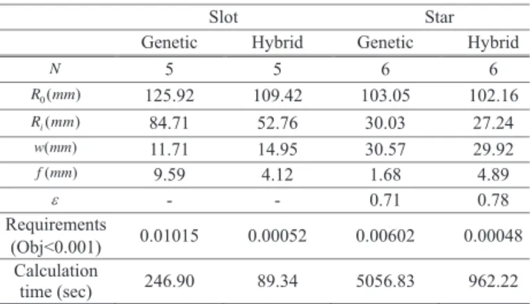
N 5 5 6 6 0( ) R mm 125.92 109.42 103.05 102.16 ( ) i R mm 84.71 52.76 30.03 27.24 ( ) w mm 11.71 14.95 30.57 29.92 ( ) f mm _9.59 _4.12 _1.68 _4.89  _- _- _0.71 _0.78 Requirements (Obj<0.001) 0.01015 0.00052 0.00602 0.00048 Calculation time (sec) 246.90 89.34 5056.83 962.22

_p 1134.75 _{kg m}_/ 3

 _8e-5

n 0.23

t

A 4.91e-4 _m2

variables

Case 1 Case 2

Initial

N 5 6 5.49 4 3.56 0( ) R mm 110 120 118.43 80 105.63 ( ) i R mm 52 50 84.71 10 11.03 ( ) w mm 15 0.5 0.44 2 -0.14 ( ) f mm 10 20 -1.87 5 14.12 - -

Generations 10

scaling window Ws 1

Variables min Max

N 4 10 0( ) R mm 50 300 ( ) i R mm 10 150 ( ) w mm 10 50 ( ) f mm 1 20  _0.01 _0.99

_p _1134.75_{kg m}_/ 3

 _8e-5

n 0.23

t

A 4.91e-4 _m2

variables

Case 1 Case 2

Initial

N 5 6 5.49 4 3.56 0( ) R mm 110 120 118.43 80 105.63 ( ) i R mm 52 50 84.71 10 11.03 ( ) w mm 15 0.5 0.44 2 -0.14 ( ) f mm 10 20 -1.87 5 14.12 - -

Generations 10

scaling window Ws 1

Variables min Max

N 4 10 0( ) R mm 50 300 ( ) i R mm 10 150 ( ) w mm 10 50 ( ) f mm 1 20  _0.01 _0.99 (780~787)2017-58.indd 784 2018-01-06 오후 7:15:16

(6)

785

http://ijass.org shortcomings.

The design variables and requirements of the hybrid optimization design have been set as shown in Table 6. By analyzing the result of the genetic algorithm, the degradation of the search performance has been identified and global requirements as the termination condition of global optimization have been set 0.01 for the slot shape and 0.011 for the star shape, respectively. Since the variables N and ε have a large influence on trend of the thrust profile, they are determined in the global solution search process of the hybrid optimization technique and the remaining variables are determined in the local optimization of it [17]. Similarly,

local requirements as the termination condition of the local optimization have been set 0.001 for the both cases.

Figures 9 for the slot shape and 10 for the star shape show the thrust profiles calculated in the optimal design process using the hybrid optimization technique. Fig. 11 shows the propellant grain configurations of the global and local solutions. In both cases, the calculated results are almost identical to the target thrust profile, and the optimized grain configurations to realize the target thrust profile are proposed. It can be confirmed that the grain design satisfying the requirements has been identified by means of the hybrid optimization technique, such that the result of the internal ballistic analysis is almost the same as the target thrust profile. In addition, as shown in Figs. 12 and 13, it has been compared with the genetic algorithm calculation process. When the hybrid optimization technique is applied to each case, both the global and the local requirements are satisfied, and the computation time is much less than with the genetic algorithm. That is, the optimum design satisfying the requirements has been found by the hybrid optimization technique.

Table 7 compares the configuration variable design results of the genetic algorithm and the hybrid optimization technique. With the hybrid optimization technique, the

11

local optimization of it [17]. Similarly, local requirements as the termination condition of the local optimization have been set 0.001 for the both cases.

Global optimization variables N R R w f, , , , ,0 i 

Local requirements Obj < 0.001 Slot grain design condition Global requirements Obj < 0.010

Star grain design condition Global requirements Obj < 0.011

Fig. 11. Grain configuration (global and local optimization)

Fig. 9. Thrust profile (Slot)

11

Fig. 10. Thrust profile (Star)

11

12

Figures 9 for the slot shape and 10 for the star shape show the thrust profiles calculated in the optimal design process using the hybrid optimization technique. Figure 11 shows the propellant grain configurations of the global and local solutions. In both cases, the calculated results are almost identical to the target thrust profile, and the optimized grain configurations to realize the target thrust profile are proposed. It can be confirmed that the grain design satisfying the requirements has been identified by means of the hybrid optimization technique, such that the result of the internal ballistic analysis is almost the same as the target thrust profile. In addition, as shown in Figs. 12 and 13, it has been compared with the genetic algorithm calculation process. When the hybrid optimization technique is applied to each case, both the global and the local requirements are satisfied, and the computation time is much less than with the genetic algorithm. That is, the optimum design satisfying the requirements has been found by the hybrid optimization technique.

Fig. 12. Objective function (Slot)

(7)

₇₈₆

calculations are completed within 90 seconds for the slot shape and within 970 seconds for the star shape, even if the requirements (0.001) are fully satisfied. A single optimization design using only the genetic algorithm has designed configuration variables similar to those of the hybrid optimization technique, but it has taken much computation time without satisfying the requirements, while the hybrid optimization technique has quickly performed the optimum design satisfying the requirements. Therefore, the hybrid optimization technique is a fast and powerful method that can be used for the optimal design of the grain configuration variables.

5. Conclusion

Grain configuration variables have a complicated effect on SRM performance and configuration variable design is a nonlinear global optimization problem with many local solutions. Optimization technique has been applied to the grain performance analysis program in order to develop a program for optimizing the configuration variables of propellant grains of the SRM. The optimum design program has consisted of a grain burn-back analysis module, internal ballistic analysis module, and optimization module. The

grain burn-back analysis module used a two-dimensional analytical technique, and a nondimensional internal ballistic analysis module has been used to calculate motor performance. The optimization module searches for configuration variables satisfying the requirements.

Deterministic optimization and stochastic optimization techniques, the simplex method and the genetic algorithm, respectively, have been applied to configuration variable optimization, but failures have occurred because of the disadvantages of each optimization technique. The deterministic optimization does not know the proper starting point of the design, and the search performance of the stochastic optimization worsens after approaching the optimum design point. In this study, a hybrid optimization technique which solves these problems by combining the optimization techniques has been developed and applied to the design optimization of grain configuration variables.

The hybrid optimization technique searches for the vicinity of the optimal point by using the genetic algorithm, and then converts it into the simplex method to calculate the correct optimal point. This process uses the advantages of each optimization technique and offsets their shortcomings.

The hybrid optimization technique has been applied to optimal design of slot- and star-shaped grains to obtain optimum grain-configuration design variables that satisfy the requirements. As a result, a more satisfactory calculation time and better design variables have been obtained than when the optimization techniques have been applied separately. Therefore, it has been verified that the hybrid optimization technique is an effective method to perform grain optimal design. In future work, the developed hybrid optimization technique will be applied to obtain optimal configuration variables of the complex geometry of multiple composition grains.

Acknowledgement

This work is supported by the Inha University Research Grant, KOREA. We would like to thank Lee Gang-gyu and Yang Sungmin for organizing the data.

References

[1] Brooks, W. T., “Solid Propellant Grain Design and Internal Ballistics”, NASA SP-8076, 1972.

[2] Nisar, K. and Guozhu, L., “Design and Comparative Study of Various Two-Dimensional Grain Configurations Based on Optimization Method”, Asian Joint Conference on Table 7. Constraint condition and requirements

Global optimization variables N R R w f, , , , ,0 i

Local requirements Obj < 0.001 Slot grain design condition

Global requirements Obj < 0.010 Star grain design condition

Slot Star Genetic Hybrid Genetic Hybrid

N 5 5 6 6 0( ) R mm 125.92 109.42 103.05 102.16 ( ) i R mm 84.71 52.76 30.03 27.24 ( ) w mm 11.71 14.95 30.57 29.92 ( ) f mm 9.59 4.12 1.68 4.89  - - 0.71 0.78 Requirements (Obj<0.001) 0.01015 0.00052 0.00602 0.00048 Calculation time (sec) 246.90 89.34 5056.83 962.22 12

Figures 9 for the slot shape and 10 for the star shape show the thrust profiles calculated in the optimal design process using the hybrid optimization technique. Figure 11 shows the propellant grain configurations of the global and local solutions. In both cases, the calculated results are almost identical to the target thrust profile, and the optimized grain configurations to realize the target thrust profile are proposed. It can be confirmed that the grain design satisfying the requirements has been identified by means of the hybrid optimization technique, such that the result of the internal ballistic analysis is almost the same as the target thrust profile. In addition, as shown in Figs. 12 and 13, it has been compared with the genetic algorithm calculation process. When the hybrid optimization technique is applied to each case, both the global and the local requirements are satisfied, and the computation time is much less than with the genetic algorithm. That is, the optimum design satisfying the requirements has been found by the hybrid optimization technique.

Fig. 13. Objective function (Star)

Study of Hybrid Optimization Technique for Grain Optimum Design

780

Paper

Study of Hybrid Optimization Technique for Grain Optimum Design

Seok-Hwan Oh*, Yong-Chan Kim*, Seung-Won Cha*, and Tae-Seong Roh**

Abstract

Nomenclature

1. Introduction

781

2. Optimal design of Solid rocket motor

2.1 Optimal design process of grain configuration

2.2 Grain burn-back analysis module





















































782

































































2.3 Internal ballistic analysis module

 

 

 

 

 

 

2.4 Optimization module



Seok-Hwan Oh, Yong-Chan Kim, Seung-Won Cha*, and Tae-Seong Roh**

₇₈₂

₇₈₄

₇₈₆