969
Copyright ⓒ The Korean Institute of Electrical Engineers
Prediction of Galloping Accidents in Power Transmission Line Using
Logistic Regression Analysis
Junghoon Lee*, Ho-Yeon Jung*, J.R. Koo**, Yoonjin Yoon* and Hyung-Jo Jung
†Abstract – Galloping is one of the most serious vibration problems in transmission lines. Power lines can be extensively damaged owing to aerodynamic instabilities caused by ice accretion. In this study, the accident probability induced by galloping phenomenon was analyzed using logistic regression analysis. As former studies have generally concluded, main factors considered were local weather factors and physical factors of power delivery systems. Since the number of transmission towers outnumbers the number of weather observatories, interpolation of weather factors, Kriging to be more specific, has been conducted in prior to forming galloping accident estimation model. Physical factors have been provided by Korea Electric Power Corporation, however because of the large number of explanatory variables, variable selection has been conducted, leaving total 11 variables. Before forming estimation model, with 84 provided galloping cases, 840 non-galloped cases were chosen out of 13 billion cases. Prediction model for accidents by galloping has been formed with logistic regression model and validated with 4-fold validation method, corresponding AUC value of ROC curve has been used to assess the discrimination level of estimation models. As the result, logistic regression analysis effectively discriminated the power lines that experienced galloping accidents from those that did not.
Keywords: Galloping, Prediction, Interpolation, Logistic regression
1. Introduction
In general, galloping refers to the severe vertical or horizontal self-excited vibration of a structure. Conductor galloping refers specifically to the oscillation of overhead power lines due to the physical properties of the line itself and wind or other local weather conditions. More specifically, galloping phenomenon has been researched to be induced by complex interactions of aerodynamic instability and iced overhead transmission lines, which can produce lift force on conductors with the formation of the bluff body and separated flow [1]. Conductor galloping often includes high-amplitude and low-frequency vibration in both the horizontal and vertical directions [2]. Such a large amplitude induced by galloping is often sufficient to cause the conductors to make contact, causing flashovers and mechanical defects. In some reported severe cases, contact between two or more power lines due to violent galloping caused the electrical current failure or a sudden drop in voltage, which activated protection relay and cut off the local supply of electricity [2]. The forceful motion of galloping can also dramatically increase the loading stress of the insulators and pylons, increasing the risks of mechanical failure and permanent breakdown of the
transmission system. Thus, galloping accidents has the potential to cause severe social and economic damages.
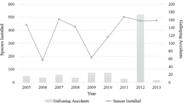
Installing anti-gallop interphase spacers is the most efficient way to prevent accidents related to galloping in power lines [3]. However, despite the substantial efforts dedicated to reducing galloping phenomena throughout South Korea, the number of reported annual galloping events has not decreased over the past decade (Fig. 1) [4] suggesting that the spacers are not being efficiently utilized. Furthermore, installing spacers in all sections of transmitting conductors without regard to galloping frequency is an inefficient and costly strategy. Therefore, the accurate prediction of accidents induced by galloping based on the internal and external conditions of a certain location is an important task for engineers when deciding where to take preventive actions.
† Corresponding Author: Dept. of Civil and Environmental Engineering, KAIST, Korea. ([email protected])
* Dept. of Civil and Environmental Engineering, KAIST, Korea. ({jhlee07, soulpower, yoonjin}@kaist.ac.kr)
** KEPCO Research Institute, Korea. ([email protected]) Received: September 8, 2016; Accepted: January 3, 2017
Fig. 1. Number of interphase spacers installed and number
Conductor galloping was recognized as a significant problem in the United States in the 1900s. Since then, many engineers have started their research on galloping phenomenon with considering the effect of wind lift forces and shape of transmission line. Subsequently, Den Hartog verified that power line instability depends on the relationship between lift force and drag force; a power line is unstable when the rate of decrease of lift force is smaller than that of drag force [5]. After a few decades, use of computer simulation began to be applied and Gawronski used it to predict the aerodynamic forces and strengths of cables in order to address galloping [6]. Shortly later, finite element method (FEM) began to be applied in the problem, and Keutgen validated FEM of galloping with benchmark cases which results obtained from wind tunnel [7]. Kermani et al. have simulated cyclic stresses of transmission lines with effect of atmospheric ice accretion [8]. Similarly, with including effect of ice accretion on multiple bundle conductors, Jing et al. have numerically investigated galloping of iced quad bundle conductor [9]. After research of several years, the factors that induce galloping were found to be the followings. For physical factors, the horizontal tension of the line, span length, structural damping, type of terrain, and type of conductor bundle were found to be crucial. For local weather factors, shapes and thickness of ice accretion, wind speed, and wind angle of attack, temperature and etc. were found to be important factors for galloping accidents. Nowadays, research of galloping with more precise simulation of effect on ice are ongoing.
However, to date, no studies have used statistical methods to predict conductor galloping accidents. Many recent studies have used statistical variables to predict such predict catastrophic events. Although many of the studies related to catastrophic events have focused on analysis and prevention, the development of machine learning techniques allowed some investigations to estimate the probability of events using statistical or machine learning methods. For example, Tehrany et al. have used decision tree method to predict flood susceptible areas and have resulted in up to 90% accuracy in validation [10]. M.-L. Guillerminet have used decision tree to predict the case of the possible collapse of the West Antarctic Ice Sheet [11]. Dieu et al. employed spatial prediction models to predict shallow landslide hazards with support vector machine (SVM), logistic regression, and various machine learning methods. Dieu et al. also reported methods for the estimation and prevention of landslide and wildfires using data-mining method [12]. Furthermore, in engineering field, R. Diao et al. have used logistic regression and decision tree method to assess security systems that can result in voltage collapse [13]. Also, Kankar et al. used artificial neural network and support vector machine to predict failures in ball bearings [14]. As can be seen, machine learning methods are widely used in a variety of fields for predicting catastrophic events. Thus, the prediction of
galloping accidents using statistical machine learning is expected to become a new area of research in the electrical and civil engineering fields.
In order to predict accidents induced by galloping phenomenon, it is important to clarify the inducing factors of galloping phenomenon. As it is widely researched in former studies, local weather factors and physical factors of power transmission systems itself are the major factors of galloping induced accidents. In the case of local weather factors, the data are available from Korea Meteorological Administration (KMA) in the form recorded by Automatic Weather Station (AWS), spread out in the nation. However, considering that the number of transmission tower intervals outnumbers the number of installed AWSs, for more specific local weather data, the recorded data must be interpolated before predicting accidents induced by conductor galloping. In the case of physical factors of the transmission system, Korea Electric Power Corporation (KEPCO) is the provider. However, the number of variables is too large for statistical machine learning, which can lead to overfitting and inaccuracy of results, the selection process in prior is mandatory. In such selection, histogram analyses have been used.
In this study, accidents induced by conductor galloping ware predicted using a statistical machine learning techniques, logistic regression analysis. Many engineers have accounted galloping phenomenon and have taken preventive actions at the designing degree of transmission towers (e.g. effect on tower geometry), however, accidents by galloping still occur. This study aims to predict accidents by galloping rather than just galloping phenomenon itself. Logistic regression was chosen among the numerous statistical machine learning techniques, such as SVM, decision tree, random forest, and neural networks, because the output variable takes the form of binary variable and also each inducing factor of galloping accidents take linear relationship with galloping, e.g. longer the span length, higher the galloping accident possibility. Also, other techniques often require much larger data pools than providers can give for this study and thus removed. The statistical machine learning approach to predict accidents induced by galloping is expected to allow electrical engineers to identify specific places on transmission wires where galloping is likely to occur under certain conditions; these predictions can be used to determine where to install anti-galloping devices like interphase spacers or where to inspect and keep maintenance levels at high in areas prone to galloping to prevent fatigue problems in all sorts of line components.
2. Theoretical Background
2.1 Logistic Regression
method that explains the relationship between qualitative dependent variables and independent variables. LRA is also widely used to estimate the probability of occurrence for a certain event through the linear combination of independent variables. The independent variables can also have quantitative values; thus, LRA is similar to linear regression in that it uses a linear combination of independent variables to explain the results. However, for qualitative dependent variables, LRA is more suitable for classification than regression.
LRA differs from simple linear regression in two main ways. First, in LRA, the range of dependent variables is limited to [0, 1] when the dependent variable is dichotomous. Second, the dependent variable follows a binomial distribution rather than a normal distribution since the dependent variable is binary. In simple linear regression, when the dependent variable is binary (only zero and one), the value of the dependent variable might be larger than one, decreasing the prediction accuracy. To solve this problem, a continuous increasing function with a value in the range of [0, 1] was proposed as link function. The link function in this text represents the overall function of logistic regression and thus it is often plotted for visual analysis. There are several link functions that can be used; logistic model, Gumbel model, Probit model and etc. In this study, as the purpose of the study was to predict the galloping phenomenon, for time efficiency, logistic model has been selected and it takes the form of
( ) 1 x x e g x e = + (1)
The basic equation of LRA is given as
0 1 1 2 2 log 1 k k p x x x p β β β β ⎛ ⎞ = + + + + ⎜ ⎟ − ⎝ ⎠ " (2)
where p is the probability of the dependent variable to happen, β is a constant, 0 β1~β are logistic regression k
coefficients, and x1~xk are independent variables used
in LRA [15]. Thus, the probability is represented as
1 1 log ( ) 1 i i i X p it X e β β − − ⋅ = ⋅ = + (3) 2.2 ROC curves
After a decision-making process is performed, the accuracy of the derived model should be evaluated. Since a receiver operating characteristic (ROC) curve illustrates the binary classification results for varying threshold values, this curve was used herein to compare the classification results obtained using LRA and SVM methods.
In an ROC curve, one axis corresponds to true positive rate (TPR, also known as sensitivity), and the other to false positive rate (FPR, also known as 1 minus specificity).
Thus, each point in the curve represents the ratio of TPR to FPR for a given selection criteria. In general, the closer the curve follows the left and the top border, the more accurate the binary classification. A curve that approaches 45 degrees indicates that the test cannot classify two results and is therefore meaningless.
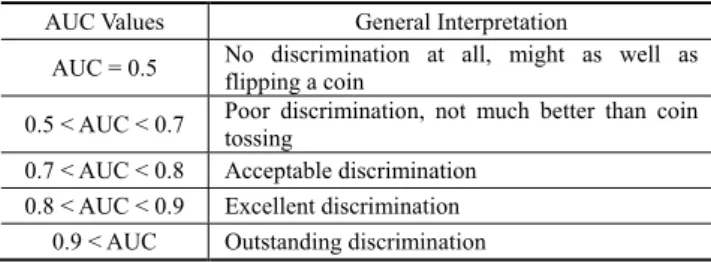
In the same manner, the accuracy of a binary classi-fication test can be evaluated based on the area under the ROC curve, widely known as AUC. As mentioned in the previous paragraph, a test can be said to be accurate when the curve is close to the top and the left border; that is, an AUC value close to 1 indicates an accurate test. Thus, the AUC value provides a measure of the model’s ability to discriminate between the subjects that experience the outcome of interest from those that do not. Table 1 lists the general interpretations of AUC values; however, there is no magic number that guarantees that the model is reliable; this depends on the tolerance of the designer.
Even if the AUC value of the ROC curve is close to 1, another important task remains: choosing the optimal threshold value. Generally, the optimal threshold value is chosen as the point at which the Youden index (i.e., sensitivity + specificity –1) is maximized (i.e., the sum of true positive and negative portions is maximized). In this study, the ROC curve and its AUC value were used to assess the accuracy of the derived model.
2.3 Histogram correlation analysis
Histogram is a simple visual or graphical representation of the distribution of numerical data and is often interpreted as bar shaped expression of a frequency table. Often, longitudinal axis of histograms represents classes or values of classes, known as ‘bin’, and vertical axis represent the corresponding frequency or count of the members.
Correlation analysis are often used in statistics to figure out how much of linear relationships exist between two different variables; two analyzed variables must be independent of each other. To explain the amount of correlation of these two comparison targets, correlation coefficient is used in general.
In this dissertation, since there lies need for comparing histograms, the correlation analysis for histograms are mandatory. However, because correlation coefficients are mainly used for two statistical variables only, a new approach is needed. Therefore correlation of histograms
Table 1. General interpretations of AUC values
AUC Values General Interpretation
AUC = 0.5 No discrimination at all, might as well as flipping a coin 0.5 < AUC < 0.7 Poor discrimination, not much better than coin tossing 0.7 < AUC < 0.8 Acceptable discrimination
0.8 < AUC < 0.9 Excellent discrimination 0.9 < AUC Outstanding discrimination
represented as metric d H H . ( 1, 2) 1 1 2 2 1 2 2 2 1 1 2 2 ( ( ) )( ( ) ) ( , ) ( ( ) ) ( ( ) ) i i i H i H H i H d H H H i H H i H Σ − − = Σ − Σ − (4)
where H and 1 H represent two comparison targets, 2
histograms and H represent k
1 ( )
k j k
H H j
N
= Σ . With
this mathematical representation, closer the value of Eq. (4) to one, has meaning of highly correlated histograms and closer to zero means no correlations at all.
3. Data Preparation
It is important to complete an extra step before estimating the occurrence of galloping accidents on transmission lines. This step is to filter useless or meaningless data out of all the weather and physical data that have been provided by KMA and KEPCO. Although from the former researches, it can be easily found that wind characteristics, shapes of ice accretion, span length, conductor bundle type and many more can be found as a direct cause of galloping phenomenon, since this study deals with predicting accidents induced by galloping with statistical machine learning technology, all of the variables should be taken in consideration, not just the ones which makes sense.
It seems logical that the more data or parameters that the system takes in, the better the accuracy or reliability of the outcome; however, an overflowing pool of parameters can result in overfitting, and the complexity of the computation process increases exponentially with the number of parameters used in the model. In addition, some variables negatively affect the prediction system when all variables are used together. Finally, failing to sort variables that are related to each other (e.g., temperature and ice accretion) can produce inaccurate results. Due to these inefficiencies, data handling is an essential pre-estimation process. This section discusses the raw data and the selection of weather and physical variables for further prediction of galloping accidents.
3.1 Raw data
Local weather data from the AWS, which collect 13 weather parameters for specific locations, were provided by the Korea Meteorological Administration. Out of the 13 parameters, only four (temperature, precipitation, wind speed, and wind direction) were considered in this study since the other factors (e.g., soil temperature and amount of daylight) have little or no influence on galloping phenomena. Also, another parameter, timely standard deviation of wind speed for past 10 minutes, has been made for making up the reason that the AWS sensor of wind direction warns about its inaccuracy. Since the data collected were not for the exact locations of accidents, the
number of transmission line intervals exceeds 50,000 while the number of AWSs installed is only 676, interpolation methods must be employed to utilize the data in predictive models. Out of numerous spatial interpolation techniques, Kriging method has been used for interpolation.
Total 122 physical variables were obtained from KEPCO: 49 for the front transmission tower, 49 for the back transmission tower, and 24 for the power line. In numbering the transmission towers, the tower with lower number is called the front tower and vice versa; for example, when a tower of interest has number 123, adjacent tower of having the number 122 is the front tower and 124 is the back tower. However, even though no special physical meanings exist with front and back tower naming, in this study, both adjacent towers just next to the tower of interest are considered differently as there are a few differences in physical factors.
Before using several methods to eliminate meaningless variables, among 122 raw variables, those which were thought to be independent with galloping were removed (e.g. number of tower, name of company of production, etc.), and variables among power lines that had relations with interphase spacers were eliminated before applying any statistical methods. This procedure eliminated 29 variables; thus, the following selection procedures were carried out on 93 physical variables, 43 each for front and back towers, 7 for power line.
The physical variables of the power-transmission devices were provided by Korea Electric Power Corporation (KEPCO), but due to security issues, the variable names are not allowed to be cited in the dissertation and thus the numbering will take place instead of variable names, e.g. pv106(pv stands for abbreviation of physical variable). The naming of physical variables is as follows; for front tower the number starts with one, for back tower, two, and for power line three, e.g. pv102 for front tower, pv202 for back tower variable, and pv304 for power line variable. Also, because of the large number of parameters, we employed a pre-estimation reduction process using variable-elimination methods.
3.2 Variable selection process
As mentioned in the introduction, the crucial inducing factors of galloping accidents must be determined in order to construct a prediction model. From former studies, the local weather factors are mandatory, no study can be found which deals the wind and ice accretion out of the system of interest. Therefore, the weather factors will be taken into consideration in the last section of the variable selection process, and physical factors will be reduced in prior.
3.2.1 Histogram analysis
As mentioned, 93 critical physical variables of power transmission systems that should be taken in consideration
for estimating galloping, including overlapping physical variables of front and back towers and that of transmission lines’. Generally, as two towers, front, back towers of accidental transmission line, are adjacent to each other, the physical properties of them can be considered to be similar. From this fact, histogram analysis of front and back towers for all physical variables of accident cases were conducted in order to find out correlations of variables in both towers, especially in the cases of accident. In this process, the overlapping variables of front and back towers showing low correlation can be understood to have different meanings, thus, variable of high correlation value of both front and back tower are necessary removed. The cutoff value has been set to 0.99.
From the result of this correlation analysis of two histograms, front and back tower, by using a value of 0.9 for cutoff criteria, only five of overlapping physical variables have been found to be necessary for using both front and back tower. The rest of physical variables have shown correlation values equal to one and therefore unneeded for them to belong in front and back tower categories, thus only that of front tower have been used. From this moment, only the five sorted out variables will be used for physical variables of back towers, while the number of physical variables of front towers, 43, remain the same for the rest of the process.
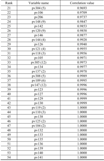
Second histogram analysis should be taken for physical variables of accidental towers and normal towers which are almost 50,000 towers. All physical variables, for both accident tower and normal towers, were made into histograms, then correlation analysis of two histograms took place, varying physical variables. Physical variables used in this histogram analysis are as follows; 43 physical variables from front tower, five variables from back tower, and seven power line variables. In this process, the analysis result of showing high histogram correlation of a certain variable was thought as having little or no discriminating effect for estimating galloping phenomenon; therefore, removed from further consideration. The cutoff value of 0.99 was set to remove highly correlated physical variables. The remaining physical variables after this histogram correlation analysis is given in Appendix. Variable names with parentheses represent categorical variables, and numbers in the parenthesis are the number of corres-ponding categories.
As the result, 27 variables were selected in this process with same cutoff criteria, 0.99. Along with the first histogram correlation analysis, which compared correlation between front and back tower, total 27 physical variables, 17 of front towers, five of back tower, and five of transmission lines, were selected out to be carried on to the next step of variable selection. From this step, it can be recognized that all five physical variables of back towers have survived and thus physical variables of back towers show correlation to galloping phenomenon. The five corresponding variables of front towers have also remained,
however, the remained categories of the categorical variable, pv111 and pv211 differ, which states that some categories of pv111 and pv211 have different correlation to galloping phenomenon.
3.2.2 Univariable logistic regression
After the histogram analyses were employed to select variables that are influential in galloping, univariable logistic regression was applied to reduce the number of less-meaningful variables. Dummy variables were included in this process as they are required for categorical variables. Dummy variables in logistic regression take either value of zero or one, in order to indicate the absence or presence of some categorical effect that may be expected to shift the outcome. The dummy variable in this regression process, the dummy taking value of zero will cause that variable's coefficient to have no role in influencing the dependent variable.
After putting dummies for categorical variable, univari-able logistic regression has been processed. The univariunivari-able logistic regression computes p-values for all variables; the p-value represents the probability of obtaining a result equal to or more extreme than the actual observed outcome. In general, the smaller the p-value, the more significant relation that the variable has to a certain event. In this process of variable elimination, the cutoff p-value was set to 0.1, and the variables that showed p-value of 0.1 or more have been eliminated.
From this process, five of front tower variables, two of back tower variables, and one of transmission tower variables have been removed, leaving total 19 physical variables. Interesting fact in the process is that the same variables of front and back towers have disappeared, (pv106, pv206) and (pv115, pv215). Although five of overlapping physical variables of front and back towers showed low correlations from the histogram analysis and considered as different variables, two of them showed low correlation with galloping phenomenon itself. Also, the categorical variable pair of overlapping five front and back variable, (pv111, pv211) showed quite a decrease in their number of categories after univariable logistic regression. As categories of pv211 remain as twice as much as pv111, it implies that the correlation of back towers with galloping accident is higher than that of front towers. This interpretation shows a thread of connection with p-value analysis since the p-value of pv211 shows lower values than pv111.
Additional logistic regression analysis has taken place after univariable logistic regression for a more specific selection of variables with the rest of 19 variables. Logistic regression analysis with single variable can result in a very low p-value itself, however, when all independent variables are taken in consideration, the resultant effect of a selected variable can be ignorable. Therefore, logistic regression all remaining independent variables must be conducted. The
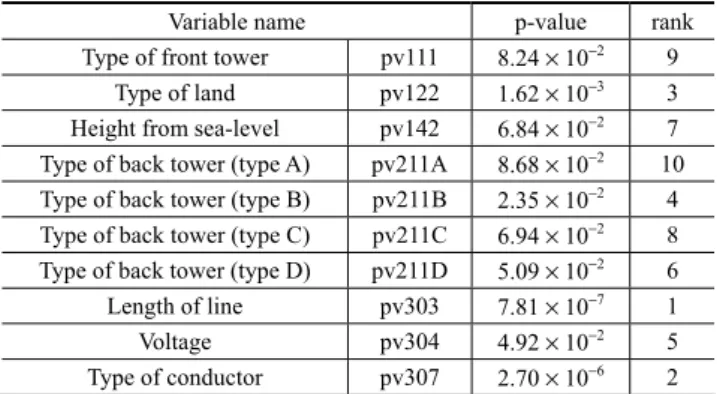
cutoff p-value of this additional logistic regression analysis was also set to 0.1 and the variables resulting in higher p-value were removed. The result of this logistic regression showing survived physical variables is shown in Table 2. The alphabets in the name of types for pv211 are just temporary.
From the result, length of transmission line showed the lowest p-value and thus can be concluded that it is the most critical physical variable. Recalling the mechanism of galloping phenomenon, as the lines experience Aeolian vibration due to various external conditions, the larger the displacement of transmission line the higher probability of the line to collide each other and induce larger dynamic stresses to other power transmission systems. Also the longer line is taken for granted that it charges more load or stress to other supporting components, leading to a higher probability of part failure when galloped. Therefore, from these reasons, it is plausible that the length of line should take its first place in p-value.
Also the type of conductor can have great meaning in galloping phenomenon in the aspect of experiencing wind pressure, especially when large amount of ice is accreted to the transmission line. As the forcing wind pressure increases along the line, the action of bluff body behind the ice and line along with effect of separated flow must also increase, risking the corresponding transmission line to gallop, as discussed in Section 1.2. The coefficient beta in the formed logistic regression model shows negative value since the pv307 represents category of single conductors; from this, multiple conductors such as quad-conductor can be interpreted to be more vulnerable to galloping phenomenon.
From the five separated variable pairs of front and back towers, that only one out of five pairs has made its way through the variable selection processes, (pv111, pv211). Even though the correlation this pair of accidental and normal cases were not in significant position, it can be now concluded that the type of transmission towers, especially those of back towers, come as important factors for galloping.
3.2.3 Backward elimination
Now, as the number of physical variables have been reduced to seven, with seven physical variables and interpolated five weather variables, backward elimination process has been conducted. Backward elimination was employed to get rid of variables that were concluded to lower the prediction performance. The Akaike Information Criterion (AIC) values of the logistic regression models were calculated to assess the suitability of the variables for further study. The AIC value is another measure of the relative quality of a statistical model. AIC value can be used to check the quality of a model, particularly in comparison to other models; thus, AIC values are typically used in the selection of models. Based on information theory, the AIC values provide the quantity of lost information when a given model is used. However, it only determines the relative quality of the model; that is, no absolute quality indicator can be computed. Thus, if all the models were either good or poor fits to the data, the AIC values would not provide any useful information. Generally, when a set of candidate models is given, the model showing the minimum AIC value is taken as the preferred model.
The remaining 12 variables were used to form logistic regression models, and the AIC values of these models were then computed by taking out each and every one of the variables. If the AIC value increased after removing the variable, that variable was removed from the dataset. This backward elimination algorithm stopped when no variable removal resulted in an increase in the AIC value. The initial AIC values of the model containing 12 variables was 699.72, whereas the final AIC value of the final model, which contained 10 variables, was 342.83. Totally removed variables are wind angle and type of front tower, and one category of the type of back tower has been removed.
3.3 Discussion
The physical factors for inducing galloping were reduced to a total of six variables: two continuous variables and four categorical variables. An interesting fact is noticed when observing the disappearing pairs of front and back tower variables. As seen from step to step, the same overlapping physical variable pairs of front and back towers get removed together, and no cases show that only one of the pairs get removed alone. Therefore, even though five pairs of overlapping physical variables were considered separately for front and back transmission towers because of their low histogram correlation, it can be concluded that the effect of the correlation was not as crucial, and thus has little meaning for selecting out physical variables. However, the pair (pv111, pv211) should be taken as an exceptional case since different number of categories have made through the selection process, making pv111 and pv211 as distinctive influential
Table 2. Result of final physical variable selection through logistic regression analysis
Variable name p-value rank Type of front tower pv111 8.24 × 10⁻² 9
Type of land pv122 1.62 × 10⁻³ 3
Height from sea-level pv142 6.84 × 10⁻² 7
Type of back tower (type A) pv211A 8.68 × 10⁻² 10
Type of back tower (type B) pv211B 2.35 × 10⁻² 4
Type of back tower (type C) pv211C 6.94 × 10⁻² 8
Type of back tower (type D) pv211D 5.09 × 10⁻² 6
Length of line pv303 7.81 × 10⁻⁷ 1
Voltage pv304 4.92 × 10⁻² 5
players among the pairs.
From the histogram correlation analysis of accidental versus normal transmission systems, the influence of transmission line variables should be specially considered as five out of seven physical variables were selected from the process. Type of conductors (pv307) was the highest in correlation rank and length of transmission line (pv303) was the third. These two variable also showed relatively small p-values in univariable logistic regression analysis and also in additional logistic regression analysis.
Another interpretation should take place with pv116, pv124, and pv324. Due to the security issues, the name of variables cannot be mentioned in the dissertation, however, the three variables are related to installation and production date. From common sense, the older the part or older the installation date, the more it is likely to be out of function. The three variables were very high in ranking of histogram correlation, and also in the univariable logistic analysis. However, the variables disappeared as they went through additional logistic regression analysis. This fact states that the date of production or installation has correlation with galloping when it is solely analyzed, but when it comes to forming a logistic model with all other physical variables altogether, the significance of the variable decreased.
After backward elimination, it can be interpreted that the effect of dividing front and back towers for types have completely vanished since all of categories of front towers have been removed from backward elimination process. The interpretation on removed weather parameter, wind direction, can refer to accuracy problem of AWS itself. In the manual of AWS, it is stated that users should be aware of wind direction information because of high noise and relatively low resolution of degrees. However, standard deviation of wind angle has not been removed even though wind direction interpolation has shown inaccurate results. This can refer to the reason that standard deviation is a term that only deals with the change in directions, and therefore it can have certain meaning for estimating galloping.
4. Development and Validation of Statistical Model
4.1 Cases for prediction model development
Out of total 230 cases of galloping accidents occurred, 84 cases were selectively chosen for learning cases of machine learning. For the reason that galloping accidents have been recorded by KEPCO when sudden voltage drop is detected in certain sections of transmission line, not all galloping phenomena are detected, but only the accidents have been recorded. In some cases, where galloping has been recorded jointly, within a short period of time interval, the events were grouped and just counted as a single case of galloping for preventing overfitting in the prediction model. The close by galloping transmission sections and
continuous galloping transmission lines are highly likely to have similar or same weather conditions; if all of the cases are fed to learning algorithm, overfitting is highly likely to happen. Also to get rid of exceptional cases, galloping phenomena that happened during summer and early autumn seasons were neglected; since in South Korea typhoon is relatively common affair and harsh wind is accompanied by them. Therefore, the rest of the cases, 146 cases, were ignored, only leaving 84 cases to be discussed.
Since this study aims to develop a prediction model of galloping induced accidents by using statistical machine learning, besides the 84 accident cases, normal status cases where galloping accidents did not take place must also be used. It is important to notice that the number of whole available samples of transmission line statuses approaches 13 billion cases to consider in the prediction process, while the number of galloping accident cases that can be taken in consideration which is only 84. Using all of the cases for prediction process will be too complicated and burdensome. Also, even when choosing out random hundred million cases, the probability of this selected out case to contain an accident case is close to zero, and thus alternative to random choice of machine learning cases must be considered. Therefore, with a ratio of 1:10, total 840 cases of only non-accidental cases were chosen out of whole 13 billion populations, resulting in total of 924 cases, 840 non-galloping cases and 84 non-galloping cases.
4.2 Prediction procedure
K-fold validation was used for cross validation in this study. In k-fold validation, the original data are randomly divided into k subsamples of equal size. A single subsample is then removed to be used for validation, while k-1 subsamples are used for the training sets. This process is done k times so that each subsample is used for validation. In this study, k = 4; therefore, the 924 cases were divided equally into four groups, each containing 21 galloping cases and 210 non-galloping cases, and four iterations of prediction and validation were performed. This four-fold validation was performed a total of 100 times. For each four-fold validation, the cases composing each of the four subsamples were randomly chosen.
After the validation, the AUC values for learning mechanism (logistic regression in this study) has been calculated and averaged with a denominator of 400. The logistic regression method was performed for three separate variable divisions: the first division was composed of four weather factors; the second division was composed of 11 physical variables; and the third contained all fifteen variables (both weather and physical factors). The results are discussed in the following sections.
4.3 Result
10 variables. Temperature, precipitation, wind speed, and power line length showed the lowest four p-values, suggesting that these four factors are the most correlated with galloping phenomenon. The negative signs of the p-values indicate reversely correlated variables. For example, a lower temperature tends to affect galloping more than a higher temperature. After the elimination steps, categorical variables were left with only a single category, and for logistic regression, only one and zero values, binary values, were used as independent variable. For instance, only single conductor for conductor type has been left and value of one was substituted for single conductor case and otherwise 0 was substituted. Before conducting subsequent analyses, it is important to note that the 10 variables shown in Table 3 show evidence of correlation, not direct causation. Therefore, we cannot say that the selected features have a direct analytical influence on galloping.
As mentioned earlier, the variables are divided into two groups: weather factors and physical factors. The AUC value for logistic regression using weather factors was 0.9343, while that using only physical factors was 0.8173. When 10 variables were grouped together as independent variables for logistic regression, the AUC was 0.9617; that is, the classification was the best when all variables were used. An AUC value exceeding 0.8 is generally considered to indicate ‘excellent’ discrimination.
4.4 Discussion
The p-values of the 10 logistically regressed were calculated and are shown in Table 3. The weather factors took first place to third place on p-value analysis, the lowest three p-value, and thus are considered crucial parameters for the prediction of galloping. However, other high-ranking factors can also be considered significant depending on the criterion used; thus, the significance of each variable affecting the result must be determined. Especially, physical variables of transmission line, length
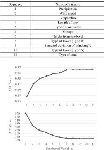
of line, type of conductor, and voltage, ranks their p-value right after the weather parameters and thus should be considered significantly. To this end, Fig. 2 plots the AUC and AIC values of each variable vs. number of variables used. The adding up sequence for variables, which follows ascending order of p-values, is shown in Table 4.
Fig. 2 shows that as the number of variables increased, the accumulative AUC value increased and the AIC value decreased, while the slope of the curve declined. Based on the point at which the AUC plot levels off, a cutoff value for the prediction can be set. In this case, it can be seen that the sharp increase in p-value occur from seventh variable, voltage. Because of security issues, the exact names of physical variables cannot be mentioned, however the lastly added 5 variables if Fig. 2 take up lower rank in correlation analysis also.
The leveling off of this curve can be explained in terms of an opportunity cost for increasing the number of variables in the model. Increasing the number of variables increases the level of complexity of the computation along with the running time of the prediction model. As seen in
Table 3. Results of logistic regression
Variable (beta values) Coefficient P-value
(intercept) -7.89 - - Temperature -0.162 1.94 × 10⁻⁷ *** Precipitation 0.202 3.71 × 10⁻¹⁶ *** Wind speed 0.768 1.03 × 10⁻⁹ *** Weather Standard deviation of wind angle 1.65 4.91 × 10⁻² * Type of land 1.21 0.165 Height from sea-level 2.08 × 10⁻³ 5.66 × 10⁻³ **
Type of tower (Type B) 0.623 8.27 × 10⁻² . Type of tower (Type D) 0.879 4.36 × 10⁻² * Length of line 4.98 × 10⁻³ 4.76 × 10⁻⁷ *** Voltage -1.51 5.58 × 10⁻⁴ *** Physical Type of conductor -2.55 1.38 × 10⁻⁶ *** Significance code: 0 ‘***’ 0.001 ‘**’ 0.01 ‘*’ 0.05 ‘.’ 0.1 ‘ ’ 1
Table 4. Sequence for variables, which follows ascending
order of p-values
Sequence Name of variable
1 Precipitation 2 Wind speed 3 Temperature 4 Length of line 5 Type of conductor 6 Voltage 7 Height from sea-level
8 Type of tower (Type B) 9 Standard deviation of wind angle 10 Type of tower (Type A) 11 Type of land
Fig. 2. Plot of AUC (upper) and AIC (lower) values vs.
the Fig. 2, first to sixth variables contribute largely for accuracy. Therefore, the number of variables used can be chosen based on the level of urgency or accuracy required. Even though some galloping occurrences might be caused by the other unknown factors, both logistic regression and SVM with the selected 10 physical and weather variables accurately estimated galloping phenomena. Thus, influencing factors other than weather and physical factors are not critical to statistically classify galloping. Thus, we can conclude that the probability model of conductor galloping is a closed system, and that the variable selection process used herein was efficient.
Stated earlier in the introduction, galloping phenomenon on conductors show high probability for several possible reasons. Since galloping phenomenon is induced by complex mechanisms of local weather parameters and physical factors of the transmission line, both of the factor groups should be taken in consideration. By case analyses done by former studies and KEPCO, most of galloping accidents occur during winter seasons when ice and snow accretion can be set on transmission lines, forming aerodynamic instability, and also a large portion of the accidental lines is affected by local wind blows, inducing Aeolian vibration motions for galloping. However, these general initiatives for galloping phenomenon are difficult to be a practical help to electrical engineers since to many exceptional cases exist. For an example of an exception, even though when a transmission line experiences ice accretion and severe wind, galloping might not be a problem if the length of the line is short enough to avoid galloping or wind blow is too irregular that it cancels out the vibration. Therefore, the prediction model constructed by machine learning techniques in this study is seen to be a practical help to the engineers in two major ways; (1) selecting out the transmission line intervals with high possibility of galloping, (2) planning a preventive scheme for future power delivery system construction.
Average number of around 300 interphase spacers have been installed annually all over the country land, but the number of galloping phenomenon does not show any consistency with the installation of spacers. From this fact, it can be concluded that even with the hard effort of preventive actions, the actual effect is small. It is evident that in the intervals where the spacers are installed, no more galloping accidents occur, and thus it can be said to be an effective action, however it leaves a room for development. By using the prediction models derived in this chapter, transmission intervals that need preferential interphase spacer installation can be selected out and the budget for preventive action of galloping can be more effectively used. Also, depending on the type of conductors or other physical properties of the transmission towers or lines, other preventive actions can be taken with the decision of KEPCO.
Secondly, for the new power intervals planned to be constructed in other areas of the country can be a practical
implication of the prediction models. With the weather data of more than 10 years a map of galloping probability can be constructed over certain areas of interest. By using this, the location of power transmission systems can be planned in prehand to minimize galloping risks. Also, by considering physical factors of transmission systems, such as the type of the tower, type of the conductor, or length of the line, reduction of galloping risks of newly constructed systems can be applied.
5. Conclusion
The reason of galloping phenomenon still remains uncertain due to the complexity of the problem itself. Until now, there have been many analytical approaches to discover the exact cause and prediction of galloping throughout the fields of engineering. However, this study has focused on rather statistical approach to predict galloping phenomenon, especially in South Korean geo-graphy, for several reasons. First, theoretical former studies and simulation attempts cannot be applied in circumstances of real world. Secondly this overall idea has been induced from several former studies of predicting catastrophic events with machine learning or data mining techniques. With such researches, events that are aroused by complex causes and mechanisms are known to be predicted with high enough accuracy. Also researches of finding more accurate result of prediction through machine learning are frequently studied with comparing newly collected data to existing experienced knowledge. But machine learning method often requires large number of data or else it may result in overfitting and unreliable outcome. Logistic regression has been chosen since it shows clear relations of independent variables and also relatively reliable when fewer data input is available.
In order to proceed in the prediction of galloping, estimation of weather parameters across the nation must be done in advance, since exact observation has not been done for every location of transmission lines. Although the exact causes for galloping are still quite unknown, many scholars and engineers have found out that local weather is the critical factor for galloping throughout the last century. Therefore, in this study, Kriging method has been implied for interpolation of total five weather factors, temperature, precipitation, wind speed, wind direction, and timely standard deviation of wind direction, that could be obtained from AWS systems provided by KMA.
Next, in prior of estimating galloping through logistic regression and SVM, variable selection process had been done. The galloping data provider, KEPCO, has provided total 122 physical variables for transmission towers. Among 122 physical variables only the meaningful variables were selected for accuracy of prediction model and time efficiency of computation. Overlapping variables and irrelevant variables such as name of manufacturing
company have been firstly removed. In order to sort out only the dominant factors, two types of histogram analyses have been conducted, front versus back tower correlation analysis, and accident cases versus non-accidental case analysis. With p-value investigation through univariable logistic regression, and multivariable logistic regression processes, only seven physical variables are found to be meaningful for predicting galloping. Before initiating the prediction process, five weather factors, previous chosen four weather factors plus standard deviation of wind direction were interpolated. Then, with chosen seven physical factors, total 12 variables have gone through backward elimination process using AIC values. As the result 10 variables, four weather variables and six physical variables have been finally chosen for independent variables of galloping prediction.
In prediction process of galloping phenomenon, the logistic regression is fed with 924 cases; 84 of galloped situation and 840 of and randomly chosen non-galloped situation from total 13 billion cases. This artificial sample selection has been done due to the remarkably low probability of contacting accidental cases when choosing sample randomly among 13 billion cases. For validation, four-fold validation has been used for total of 100 times. After the validation, the AUC values for the learning mechanism (logistic regression) were calculated. The result of logistic regression using all physical variables and weather variables has shown AUC value of 0.9617, a high AUC value compared to other classifying studies done. Whether to find out if this prediction model works for real situations, a recent case of galloping has been fed into the model; the prediction model constructed in this study does not contain the information of this newly fed galloping situation, thus another validation is possible. In this application, the probability of galloping in front, middle and back transmission lines versus time have been plotted. As the result, in the time period of galloping the probability showed values very close to one in the accident transmission line interval.
Also, AUC and AIC values of prediction model have been plotted with increasing number of variables used; the variables were added in ascending sequence of p-value, so that dominant factors are added with priority. After seventh added variable, the flattening of both curves can be found and not much of difference were found. Therefore, the addition of the variable should be thought as an opportunity cost for computational burden and accuracy. Lastly, all 84 accident cases have been checked again with the same method used in validation of recent cases, in order to find out the discrimination power of the prediction model when adjacent power lines sharing very similar physical and weather variables. As the result, AUC value of 0.7106 has been calculated, and for conclusion certain degree of discrimination is possible even with adjacent towers of similar properties.
Additional consideration of geological factors such as
land cover type, would be helpful for the more precise prediction model. However, certain factors were indefinite to select with the data that can be provided, and for this study, such geological parameters were thought to be covered with one of the physical factors, type of land. Furthermore, considering the characteristics of South Korean mountainous terrains, complex orography can be thought to be very influential to wind vectors. This consideration, however, is not contained in the inter-polation of weather parameters; the interinter-polation method considered in this study does not include the effect of terrain for weather factors and interpolated only on the plane. Therefore, advanced method of weather parameter interpolation is expected to increase the accuracy of the prediction model.
Acknowledgements
This work is financially supported by Korea Ministry of Land, Infrastructure and Transport (MOLIT) as「U-City Master and Doctor Course Grant Program」and Korea Electric Power Corporation (KEPCO) Research Institute as a service task project (R14TA02).
References
[1] Farzaneh, M., Atmospheric icing of power networks, Springer Science & Business Media, 2008.
[2] Lilien, J.-L., State of the art of conductor galloping, CIGRE, 2007.
[3] Z. K.-j. F. Dong-jie and W. J.-c. S. Na, “The Galloping and Its Preventing Techniques on Overhead Transmission Line,” Electrical Equipment, vol. 6, pp. 6, 2008.
[4] C. S. Yoon, J. R. Koo, and H. H. Sung, Prevention of Galloping Accident through Install Standard for Spacer on Transmission Power Line, Korea Electric Power Corporation, Republics of Korea, 2010. [5] J. Den Hartog, “Transmission line vibration due to
sleet,” Transactions of the American Institute of Elec-trical Engineers, vol. 4, pp. 1074-1076, 1932. [6] K. E. Gawronski and R. J. Hawks, “Computer
simul-ation of galloping catenaries,” Electric Power Systems Research, vol. 1, pp. 283-289, 1978.
[7] R. Keutgen and J.-L. Lilien, “Benchmark cases for galloping with results obtained from wind tunnel facilities validation of a finite element model,” Power Delivery, IEEE Transactions on, vol. 15, pp. 367-374, 2000.
[8] M. Kermani, M. Farzaneh, and L. E. Kollar, “The Effects of Wind Induced Conductor Motion on Accreted Atmospheric Ice,” Power Delivery, IEEE Transactions on, vol. 28, pp. 540-548, 2013.
[9] J. Hu, B. Yan, S. Zhou, and H. Zhang, “Numerical investigation on galloping of iced quad bundle conductors,” Power Delivery, IEEE Transactions on, vol. 27, pp. 784-792, 2012.
[10] M. S. Tehrany, B. Pradhan, and M. N. Jebur, “Spatial prediction of flood susceptible areas using rule based decision tree (DT) and a novel ensemble bivariate and multivariate statistical models in GIS,” Journal of Hydrology, vol. 504, pp. 69-79, 2013
[11] M.-L. Guillerminet and R. S. Tol, “Decision making under catastrophic risk and learning: the case of the possible collapse of the West Antarctic Ice Sheet,” Climatic Change, vol. 91, pp. 193-209, 2008.
[12] D. T. Bui, B. Pradhan, O. Lofman, I. Revhaug, and Ø. B. Dick, “Regional prediction of landslide hazard using probability analysis of intense rainfall in the Hoa Binh province, Vietnam,” Natural hazards, vol. 66, pp. 707-730, 2013.
[13] R. Diao, K. Sun, V. Vittal, R. J. O'Keefe, M. R. Richardson, N. Bhatt, et al., “Decision tree-based online voltage security assessment using PMU measurements,” Power Systems, IEEE Transactions on, vol. 24, pp. 832-839, 2009.
[14] P. Kankar, S. C. Sharma, and S. Harsha, “Fault diagnosis of ball bearings using machine learning methods,” Expert Systems with Applications, vol. 38, pp. 1876-1886, 2011.
[15] Menard, S., Applied logistic regression analysis, Sage, 2002.
Appendix
Table 5. Result of histogram correlation analysis; variables of accidental cases versus non-accidental cases
Rank Variable name Correlation value
1 pv307 (5) 0.6426 2 pv116 0.7227 3 pv124 0.7884 4 pv306 (12) 0.7958 5 pv115 0.8554 6 pv303 0.8653 7 pv324 0.8700 8 pv211 (20) 0.8777 9 pv213 0.8823 10 pv215 0.8919 11 pv113 0.9045 12 pv212 0.9047 13 pv114 0.9201 14 pv112 0.9268 15 pv111 (20) 0.9297 16 pv122 (16) 0.9480 17 pv102 (3) 0.9589 18 pv143 0.9647 19 pv128 (3) 0.9652 20 pv131 0.9671
Rank Variable name Correlation value
21 pv304 (5) 0.9693 22 pv106 0.9709 23 pv206 0.9737 24 pv148 (9) 0.9847 25 pv142 0.9853 26 pv120 (9) 0.9858 27 pv146 0.9877 28 pv144 (4) 0.9928 29 pv126 0.9940 30 pv121 (4) 0.9955 31 pv118 (3) 0.9956 32 pv105 0.9971 33 pv305 (12) 0.9973 34 pv134 0.9977 35 pv137 (2) 0.9978 36 pv308 (5) 0.9989 37 pv109 (6) 0.9995 38 pv147 (12) 0.9996 39 pv123 0.9996 40 pv127 0.9996 41 pv129 0.9999 42 pv130 0.9999 43 pv119 (2) 1.0000 44 pv110 (3) 1.0000 45 pv138 1.0000 46 pv125 (2) 1.0000 47 pv104 (2) 1.0000 48 pv132 1.0000 49 pv133 1.0000 50 pv135 1.0000 51 pv136 1.0000 52 pv139 1.0000 53 pv140 1.0000 54 pv141 1.0000
Junghoon Lee received B.S. and M.S.
degrees in Civil and Environmental Engineering from KAIST, Daejeon, Korea, in 2011 and 2012, respectively. He is currently working on Ph.D. course in the Civil and Environmental Engineering department at KAIST. His research interests are sensor network, structural health monitoring and big data processing.
Ho-Yeon Jung received the B.S. and
M.S. degrees in Civil and Environ-mental Engineering from KAIST, Daejeon, Korea in 2011 and 2013, respectively. Currently, he is in a Ph.D. degree at KAIST. His research interests include structural control and health monitoring.
J. R. Koo received the B.S. degree in
Mechanical Engineering from CNU, Daejeon, Korea, in 2010. His main research interest is mechanical vibrat-ion problems at power plant machines.
Yoonjin Yoon is an assistant professor
in the department of Civil and Environ-mental Engineering at KAIST. Her main research interests include data driven risk analysis and probabilistic optimization. She received her Ph.D. degree in Civil and Environmental Engineering from University of Cali-fornia, Berkeley.
Hyung-Jo Jung received the B.S.
degree in Mechanical Engineering from KAIST, Daejeon, Korea, in 1993 and the M.S. and Ph.D. degrees in Civil Engineering from KAIST in 1995 and 1999, respectively. Currently, he is a professor in the department of Civil and Environmental Engineering at KAIST. His research interests include structural control using smart materials, structural health monitoring and energy harvesting technologies.