Numerical Analysis of Vortices Behavior in a Pump Sump

저작자표시-비영리-변경금지 2.0 대한민국 이용자는 아래의 조건을 따르는 경우에 한하여 자유롭게 l 이 저작물을 복제, 배포, 전송, 전시, 공연 및 방송할 수 있습니다. 다음과 같은 조건을 따라야 합니다: l 귀하는, 이 저작물의 재이용이나 배포의 경우, 이 저작물에 적용된 이용허락조건 을 명확하게 나타내어야 합니다. l 저작권자로부터 별도의 허가를 받으면 이러한 조건들은 적용되지 않습니다. 저작권법에 따른 이용자의 권리는 위의 내용에 의하여 영향을 받지 않습니다. 이것은 이용허락규약(Legal Code)을 이해하기 쉽게 요약한 것입니다. Disclaimer 저작자표시. 귀하는 원저작자를 표시하여야 합니다. 비영리. 귀하는 이 저작물을 영리 목적으로 이용할 수 없습니다. 변경금지. 귀하는 이 저작물을 개작, 변형 또는 가공할 수 없습니다.

Master’s Thesis

Numerical Analysis of Vortices Behavior in a

Pump Sump

Supervisor Prof. Young-Ho LEE, Ph.D

August 2017

Department of Mechanical Engineering

Graduate School of Korea Maritime and Ocean University

CONTENTS LIST OF FIGURES ... VI LIST OF TABLES ... V ABSTRACT ... IX NOMENCLATURE ... XI CHAPTER 1 INTRODUCTION ... 1 1.1 Background ... 1 1.2 Previous study ... 2 1.3 Study methodology ... 3

CHAPTER 2 PUMP INTAKE DESIGN THEORY AND VORTICES FORMATION... ... 4

Introduction ... 4

Importance of pump intake design ... 4

Standard for pump intake design ANSI/HI 9.8. ... 5

Model test of intake structure ... 12

Cavitation phenomena... 23

CHAPTER 3 COMPUTATIONAL FLUID DYNAMICS (CFD) ANALYSIS AND EXPERIMENTAL SETUP ... 27

Introduction to CFD ... 27

Governing equation ... 28

Turbulence models ... 29

Cavitation models ... 32

Numerical approach ... 46

Experimental setup ... 48

CHAPTER 4 SWIRL ANGLE ANALYSIS ... 52

Swirl meter rotation ... 52

Swirl angle method ... 54

Rigid body motion ... 56

Swirl angle result ... 58

CHAPTER 5 RESULTS AND DISCUSSION ... 61

Vortices results ... 61

Results of mixed flow pump sump model ... 69

Cavitation phenomena analysis ... 72

CHAPTER 6 CONCLUSIONS ... 75

ACKNOWLEDGEMENT ... 77

List of Figures

Fig 2.1 Recommended dimensions for rectangular sump ... 6

Fig 2.2 Sump design process (ANSI/HI 9.8) ... 10

Fig 2.3 Recommended inlet bell design diameter (ANSI/HI 9.8) ... 11

Fig 2.4 Free surface vortex ... 16

Fig 2.5 Classification of vortex types ... 18

Fig 2.6 Methods to reduce submerged vortices ... 22

Fig 2.7 Technologies depend on cavitation ... 24

Fig 2.8 Variation of liquid pressure in the suction region of a pump ... 26

Fig 3.1 Two phase pump sump modeling ... 37

Fig 3.2 General meridional geometry for turbomachinery ... 38

Fig 3.3 Meridional and 3D geometry for mixed flow pump ... 39

Fig 3.4 2D drawing for pump sump with mixed flow pump ... 40

Fig 3.5 Fluid domain and structure modeling for mixed flow pump ... 41

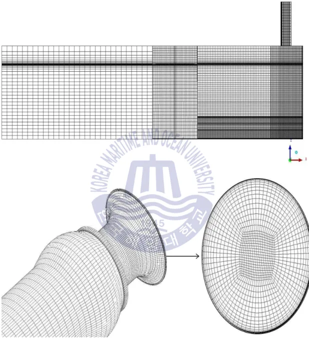
Fig 3.6 Overall mesh generation for sump model ... 44

Fig 3.7 Grid details of bell mouth and sump domain ... 45

Fig 3.8 Top view mesh generation ... 46

Fig 3.9 Mixed flow pump mesh generation ... 46

Fig 3.10 Experimental setup ... 49

Fig 4.1 Angular motion ... 53

Fig 4.2 Typical swirl meter ... 54

Fig 4.5 Swirl angle comparison ( Exp & CFD) ... 59

Fig 4.6 Tangential velocity profile ... 60

Fig 5.1 Free surface vortex types ( Exp & CFD) ... 63

Fig 5.2 Air volume fraction plane for free surface vortex (type 5 ) at different time step ... 64

Fig 5.3 Free surface vortex, helical path and pressure distribution ... 65

Fig 5.4 Velocity stream line at top surface ... 66

Fig 5.5 Tangential velocity plane ... 66

Fig 5.6 Velocity vectors for submerged vortex ... 67

Fig 5.7 Velocity plane for submerged vortex ... 67

Fig 5.8 Vorticity of sump width direction at different flow rates ... 68

Fig 5.9 Performance curve of mixed flow pump without and with sump ... 71

Fig 5.10 Cavitation region inception ... 72

Fig 5.11 Cavitation performance curves of mixed flow pump ... 73

List of Tables

Table 2.1 Recommended value for dimensions variable ... 7

Table 2.2 Acceptable velocity ranges for inlet bell diameter ... 10

Table 2.3 Parameter study on Re and We number for all cases ... 14

Table 2.4 Vortices acceptance criteria ... 20

Table 3.1 Design specification of the mixed flow pump ... 38

Table 3.2 Mesh information for impeller and diffuser ... 43

Table 3.3 Study cases ... 49

Table 4.1 Swirl angle results ... 59

Numerical Analysis of Vortices Behavior in a Pump Sump

Ayham Amin Alhabashna

Department of Mechanical Engineering

Graduate School of Korea Maritime and Ocean University

Abstract

Recently, designers and engineers of pump stations realized that the efficiency and performance of a pumping station does not depend only on the performance of selected pumps, but also on proper design of intake structure. Most recurring problems faced in a pumping station are related to the sump or intake design rather than pump design. International design standards for a pump sump restrict undesirable flow patterns up to a certain extent implication of which does not guarantee a problem free sump but provides a basis for initial design. A faulty design of pump sump can lead to form of swirl and vortex, which reduce the pump efficiency and induce vibration, noise, and cavitation. To reduce these problems and for the advanced pump sump design with high performance, it is essential to know the detailed flow behavior in sump system. Swirl angle parameter and vortices formation are important parameters that determine the quality of flow ingested by sump. According to the swirl angle parameter, the hydraulic institute prescribes the method that needs to be employed for estimating this parameter.

location, and air entrance in details. A four blade zero-pitch traditional swirl meter was installed at the suction pipe to measure the flow intensity by swirl angle calculations; the key point is to obtain the average tangential velocity at different suction pipe diameter. The other part of this study is overall numerical analysis for sump model with a mixed flow pump installed. Hydraulic performance of the mixed flow pump for head rise, shaft power, and pump efficiencies versus flow rate changed from 50% up to 150% of the design flow rate were studied by performances curves. In addition, a basic numerical simulation of cavitation phenomenon in the mixed flow pump has been performed by calculating the full cavitation model with k-ε turbulence model.

Swirl angle and average tangential velocity estimated by CFD simulation was in agreement with experimental results obtained. The results also show that submerged vortex strength was almost proportional to the flow rate in the sump. The free surface vortex had an unsteady behavior as its location and duration drastically varied. In addition, post processing results showed the tangential velocity behavior and the four types of free surface vortex (Surface swirl, Surface simple, air bubbles and full air core to intake) by changing the air volume fraction values. In the mixed flow pump performance study, the efficiency without and with sump model was 83.4% and 80.1% respectively at the design flow rate.

Key words: Pump sump, Vortices, Swirl angle, Mixed flow pump, Computational Fluid Dynamic (CFD)

Nomenclature

B Distance from the back wall to the pump inlet mm C Distance between the inlet bell and floor mm D Inlet bell design outside diameter mm

Fr Froude number -

g Gravity acceleration m/s2

Ht Total head m

n Revolution per minute rpm

P shaft Hydraulic shaft power kw

Pv Vapor pressure Pa

Q Volume flow rate /

S Minimum submergence depth m Vb Velocity at bell mouth m/s

α Angle of floor slope °

η Pump efficiency %

θ Swirl angle °

λ Scale ratio of model dimensions to prototype -

μ Viscosity Pa.s

ν Kinematic viscosity /

ρ _{Specific water density kg/m}3

σ Surface tension N/m

Introduction

Background

A pump sump or intake is simply defined as a hydraulic structure with specific dimensions used to contain the water which has to be pumped into the piping system. Ideally, the flow of water into any sump or intake should be uniform, steady and free from swirl, vortex, and entrained air. The Poor intake or wet well design may result in submerged or surface vortices, swirl of flow entering the pump, non-uniform distribution of velocity at the pump impeller and entrained air or gas bubbles, even lead to excessive bearing load, change clearances and structure damage. There are some international design guidelines for the specific geometrical and hydraulic constraints of the pump sump. One of these standards is ANSI/HI 9.8 for pump intake design, which suggests a procedure to perform scaled model tests assess the quality of flow in the intake pipe using a swirl meter and recommends the measured swirl angles to be limited to less than a prescribed limit. However the application of these standards does not generate a problem free sump but provide a basis for the initial design. For any project, the model study is the only tool for solving potential problem in new designs and rectifying problems observed in existing installations. The scaled model tests are expensive and time consuming, so alternative Computational Fluid Dynamics (CFD) methods for evaluating sump performance and flow analysis have been developed. With rapid process time in CFD, numerical simulation is regarded as an effective tool in solving fluid problems in pump sumps.

Previous study

Many researchers studied the flow conditions and undesirable phenomenon in sump intake. Lee et. al. [1] had conducted numerical analysis for the flow characteristic around pump intake by the unbalanced velocity in the direction of flow passage. Kim et. al. [2] made comparative analysis of flow behavior around intake entrance by PIV method and CFD analysis; also he studied a swirl angle of swirl meter at different types and location. Luca Cristofano et. al. [3] made an experimental study on unstable free surface vortex and gas entrainment onset condition. The main purpose of his research was to understand the influence of different parameter on free surface vortex formation and evolution. Iwano et. al.[4] have introduced numerical method for the submerged vortex by analyzing the flow in the pump sump with and without baffles plates . Oh H W [5] conducted a mixed flow pump design optimization with specific parameter and compared the numerical results with the experiments. Kim et. al. [6] made performance analysis with numerical simulation for mixed flow pump and improved the hydraulic efficiency by modification of the geometry.

Cavitation phenomenon is considered as an undesirable phenomenon caused by adverse flow condition. “Cavitation” is a process of partial evaporation of liquid in a flow system. A cavity filled with vapor is created when the static pressure in a flow locally drops to the vapor pressure of the liquid due to excess velocities, so that some fluid evaporates and a two-phase flow is created in a small domain of the flow field. With rapid formation, growth and collapse of the bubbles, cavitation

increase and even equipment damage. The cavitation phenomenon has been studied by many researchers. Okamara et. al. [7] made two CFD cavitation prediction methods used in the pump industry manufactures, and attempts were made to improve the cavitation performance. Li et. al. [8] conducted numerical analysis on the basis of the development liquid/vapor interface tracking method to predict the cavitation characteristics with a centrifugal pump impeller model. Moreover, there are a number of correlated studies [9]-[11].

Study methodology

The first part of this study will suggest the flow behavior in pump sump (swirl angle estimation, vortices prediction). For swirl angle, the objective is to estimate the swirl angle as used by Hydraulic Institute Exp and CDF, then comparison of the results will be aimed at. For vortex prediction, the aim is to predict the different types formation in the sump(free surface vortex, side wall and submerged vortex) by occurrence, location, and air entrance in details. The second part will be overall numerical analysis for sump model with a mixed flow pump installed. The hydraulic performances of the mixed flow pump will be studied by performances curves, without and with sump installation. In addition, a basic numerical simulation of cavitation phenomenon in the mixed flow pump has been performed by calculating the full cavitation model with k-ε turbulence model.

Pump Intake Design Theory and Vortices Formation

Introduction

For pumps to achieve their optimum hydraulic performance across all operating conditions, the flow at the impeller must meet specific hydraulic conditions. The ideal flow entering the pump inlet should be a uniform velocity distribution without rotation and should be stable over time. When designing a sump to achieve a favorable inflow to the pump or suction pipe bell, various sump dimensions relative to the size of the bell are required. Using these standards of the distances to reduce the probability of the occurrence of strong submerged vortices and free surface vortices.

Importance of pump intake design

The specific hydraulic phenomena that have been confirmed can lead to certain common operational problems. The main problems are summarized as follows:

• Nonuniform distribution of velocity in space and time at the impeller eye.

• Entrained air or gas bubbles.

• Preswirl magnitude and fluctuation with time.

• Free surface vortices.

• Submerged vortices.

The problems encountered in the pump sump will affect the pump performance and significantly increase the operational and maintenance cost. In order to identify sources of particular problems and find practical solutions for it, the usual approach

objectives are to ensure that a pump station is designed according to best practice and conforms to the requirements set out in the American National Standard for pump intake design [12]. These standards restrict the degree to which above-mentioned undesirable flow patterns may be present. The negative impact of each of these phenomena on pump performance depends on pump specific speed and size. The application of these standards does not generate a problem free sump but provide a basic for the initial design.

High swirl in the pump intake can cause significant change in the operation conditions for a pump, and effects on the flow capacity, power requirement and efficiency. Also it is lead to occur free surface and submerged vortices, which influence the pump capacity, impose a fluctuating load on the pump impeller blade, and may induce cavitation of the impeller blades.

Standard for Pump Intake Design ANSI/HI 9.8.

ANSI/HI 9.8 is an institute standard that defines the product, material, process or procedure with reference to one or more of the flowing: nomenclature, composition, construction, dimensions, tolerance, safety, operating characteristics, performance, quality, rating, testing, and service for which designed. The purpose of the institute is promote the continued growth of pump and intake design knowledge for the interest of the pump manufactures and to further the interests of the public in such matters that are involved in manufacturing ,engineering:

• To develop and publish standards for pumps.

• To increase the amount and to improve the quality of pump service to the public.

• To support educational and research activities.

In our study we used ANSI/HI 9.8 as a reference for all pump sumps dimensions, swirl meter location and installation sequences.

Recommended dimensions for a rectangular sump.

According to HI institute, the proportion of the inlet structure can be estimated. Fig. 2.1 and Table 2.1 shows the recommended dimensions for a rectangular sump.

Table 2.1 Recommended value for dimensions variable [12]

Dimension

Variable Description

Recommended value

h Minimum height of constricted bay section near the _{pump inlet bell} h= (greater of H or _2.5D)

H Minimum Liquid depth H=S+C

A Distance from the pump inlet bell centerline to the

entrance A=5D minimum

a Length of constricted bay section near the pump inlet 2.5D minimum

B Distance from the back wall to the pump inlet bell

centerline 0.75D

C Distance between the inlet bell and floor 0.3D 0.5D

D Inlet bell outside diameter Section 2.3.2 W Pump inlet bay entrance width W=2D minimum

w Constricted bay width near the pump inlet bell W=2D

X Pump inlet bay length 5D minimum

Y

Distance from pump inlet bell centerline to the

downstream face of through-flow traveling screen. 4D minimum

Z1 Distance from pump inlet bell centerline to diverging _walls. 5D minimum

Z2 Distance from pump inlet bell centerline to sloping floor.

5D minimum

∝ Angle of floor slope 10°~10°

β Angle of wall convergence 0°~10° ∅ Angle of convergence from constricted area to bay

wall. 10

° _maximum S Minimum pump inlet bell submergence S = D (1.0+2.3 Fr)

In a sump model a Froude number and Reynolds number are the most important non dimensional parameters. The Froude number, representing the ratio of inertial to gravitational forces, can be defined for pump intake as:

= ( ) .

(2.1)

Where:

: Froude number at D (dimensionless)

∶ Velocity at suction inlet = Flow/Area, based on D D: Outside diameter of bell or inside diameter of pipe inlet

: Gravitational acceleration

The hydraulic institute put design sequences as a reference for intake structures:

• Consider the flow patterns and boundary geometry of the body of liquid from which the pump station is to receive flow. Compare with the approach of the body of liquid from which the pump station is to receive flow. Compare with the approach flow condition described, if the hydraulic physical model study is required.

• Determine the number and size of pumps required to satisfy the range of operating conditions likely to be encountered.

• Identify pump inlet bell diameter. If final bell diameter is not available.

• Determine the required bell submergence.

• Determine the minimum allowable liquid depth in the intake structure from the sum of the floor clearance and the required bell submergence.

• Check bottom elevation near the entrance to the structure and determine if it is necessary to slope the floor upstream of the bay entrance. If the resulting depth at the entrance to the intake structure is shallow, then check to ensure that gravity-driven flow is not restricted by the entrance condition.

• Check the pump bay velocity for the maximum single-pump flow and minimum liquid depth with the bay width set to 2D. If bay velocity exceed 0.5m/s, then increase the bay width to reduce to a maximum flow velocity of 0.5 m/s.

• Compare cross-flow velocity (at maximum system flow) to average pump bay velocity. If cross flow value exceed 50% of the bay velocity, a physical hydraulic model study is necessary.

• Determine the length of the structure and dividing walls, giving consideration to minimum allowable distances to a sloping floor, screening equipment, and length of dividing walls. If dual flow traveling screens or drum screens are to be used, a physical hydraulic model study is required.

• If the final selected pump bell diameter and inlet velocity is within the range given, then the sump dimensions need to be changed and will comply with these standards.

Inlet bell design diameter

The geometry is generally defined in terms of the pump inlet diameter and Inlet bell velocity, as shown in Table 2.2 and Fig. 2.2, Fig. 2.3, the bell diameter can be estimated based on an inlet pipe velocity.

Table 2.2 Acceptable velocity ranges for inlet bell diameter [12]

Pump Flow Range Q, (L/s)

Recommended Inlet Bell Design Velocity,

(m/s)

Acceptable Velocity Range (m/s)

Q < 315 V=1.7 0.6 2.7

315 Q 1260 V=1.7 0.9 2.4

Model test of intake structure

Actually, the flow behavior in a pump sump or intake is difficult to predict by empirical formulae or traditional mathematics. For huge structures or those that differ significantly from proven design, a model study is the only means to ensure success. Usually, model study is used to identify adverse hydraulic condition and derive remedial measures for approach flow patterns generated by structures up stream of the pump impeller. The objective of a model study is to ensure that the pump intake structure generates favorable flow condition at the inlet to the pump evaluation for the requirement of model test if:

• Sump or piping geometry that deviates from the design standard.

• Non-symmetric or Non-uniform flow to the pump sump exists.

• The pumps have flows greater than 2250 L/s per pump or the total station flow with all pumps running would be greater than 6310 L/s.

• Situation that need ten times cost than model study. Similarity condition and scale effects

Similarity condition

In model test, geometric similarity at bell mouth and surrounding wall must be maintained between prototype pumps and model pumps. This is to ensure that the result obtained from the model study is well presented in order to predict full scale behavior.

By the law of similarity, the Froude number shall be equal in model and prototype.

$ = % & '% =

%

& '( (2.2)

Where Fr is the Froude number, Lm is the characteristic length of model sump and Lp the characteristic length of full scale sump.

Scale effects

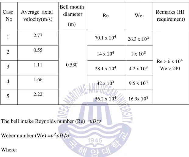
In sump model, Froude number (Fr) and Reynolds number (Re) are the most important non-dimensional parameters. But it is impossible to have all these parameter the same with prototype. Some reduction in Re should be introduced to sump model. However, flow patterns are generally very similar at high Re. The influence of viscous forces on vortex may be negligible if the values of Reynolds number in the model above 6 ∗ 10* at the suction bell mouth [12]. No specific geometry scale ratio is recommended, but the resulting dimensionless numbers must meet these values. For practically in observing flow pattern and obtaining accurate measurement, the model scale shall yield a bay width of at least 300mm, a minimum liquid depth of at least 150 mm, and pump through or suction diameter of at least 80 mm in the model. In this study, bay width is 500mm, the liquid depth is 800mm, bell mouth diameter is 530mm, all satisfying the HI standard requirement. Table 2.3 shows parametric study of model Reynolds number (Re) and weber number (We) obtained in this study. Two non-dimensional numbers satisfy Hi standards requirement for all cases, that’s mean no scale effect.

Table 2.3 Parameter study on Re and We number for all cases Case No Average axial velocity(m/s) Bell mouth diameter (m) Re We Remarks (HI requirement) 1 2.77 0.530 70.1 x 10* _{26.3 x 10} Re > 6 x 10* We > 240 2 0.55 _{14 x 10}* _{1 x 10} 3 1.11 _{28.1 x 10}* _{4.2 x 10} 4 1.66 _{42 x 10}* _{9.5 x 10} 5 2.22 _{56.2 x 10* 16.9x 10}

The bell intake Reynolds number (Re) =+ /, Weber number (We) =+ - /.

Where:

+ : Average axial velocity (m/s), : Bell mouth diameter (m), ,: Kinematic viscosity of liquid ( /s)

Vortices Formation around pump intake Overview

In fluid dynamics, a vortex is a region in a fluid in which the flow rotates around an axis line, which may be straight or curved [13]. The plural of vortex is either vortices or vortexes. Vortices form in stirred fluids, and may be observed in phenomena such as smoke rings, Pump intakes, or the winds surrounding a tornado or dust devil.

Vortices are a major component of turbulent flow. The distribution of velocity, vorticity (the curl of the flow velocity), as well as the concept of circulation are used to characterize vortices. In most vortices, the fluid flow velocity is greatest next to its axis and decreases in inverse proportion to the distance from the axis.

Cavitation phenomenon is considered as undesirable phenomenon caused by adverse flow condition. “Cavitation” is a process of partial evaporation of liquid in a flow system. A cavity filled with vapor is created when the static pressure in a flow locally drops to the vapor pressure of the liquid due to excess velocities, so that some fluid evaporates and a two-phase flow is created in a small domain of the flow field. With rapid formation, growth and collapse of the bubbles, cavitation manifests in the form of pump performance decrease, vibration, additional noise increase and even the equipment damage.

Vortices formation in pump sump

The function of an intake is basically to withdraw water safely from the source and divert this water to an intake conduit. The drawn water is mostly used for flood

control (spillway), irrigation, electric power generation and water supply. Flow through the intake is a complicated type of flow. The design of an intake is basically consists of the direction, the location and the size of the intake structure. If the intake is close to the water surface to reduce the cost, there occurs the risk of air-entraining vortex formation. If the intake structure is close to the bottom to increase the amount of water available to withdraw, there occurs the risk of sedimentation blockage. Consequently, while designing an intake structure, an optimization must be reached between the cost, safety and efficiency.

Fig. 2.4 Free Surface Vortex

There are various investigations that provide insight into the fundamental processes leading to the development of vortices both in experimental and numerical simulation. Shin et. al. [14] demonstrated two basic mechanism lead to inlet vortex formation. The first mechanism involves the development of an inlet vortex due to the amplification of ambient vorticity in the approach flow as vortex lines are convicted into the inlet. The second mechanism involves the development of a trailing vortex in the vicinity of the intake as a result of the variation in

circulation along the inlet. For this second case, a vortex can develop in a flow that is irrotational upstream, and the vortex development therefore does not depend on the pressure of ambient vorticity. Shin et. al. investigation on kinematic parameters, indicate that the strength of an inlet vortex or trailing vortex system Increase with decreasing distance from the surface. However, for an inlet in an upstream irrotational flow, two counter rotating vortices can still trail from the rear of the inlet.

Classification of vortex type

As illustrate in Fig. 2.5, vortices in the vicinity of pump intakes may be adjacent to the channel bottom or a channel wall (i.e. submerged vortices) or they may appear adjacent to the free surface (i.e. free surface vortex).

1 Su r fac e sw irl 2 Su rfa c e dim ple C oh eren t sw irl 3 D ye co r e to _{i nt ake:} c o her e n t sw irl t hro u gh ou t w ate r c o lu m n

4 V o rte x pu llin g_{flo ating t ras h} bu t n ot a ir

5 V or tex pu llin g_{air bu b bl e s to} in ta k e

6 F u ll a ir core_{to in ta ke} V ort ex

type Vort e x typ e

1 Su r fac e sw irl 2 Su rfa c e dim ple C oh eren t sw irl 3 D ye co r e to _{i nt ake:} c o her e n t sw irl t hro u gh ou t w ate r c o lu m n

4 V o rte x pu llin g_{flo ating t ras h} bu t n ot a ir

Tr ash

5 V or tex pu llin g_{air bu b bl e s to} in ta k e

6 F u ll a ir core_{to in ta ke} V ort ex

Fig. 2.5 Classification of vortex types [12]

Many researchers focused on the numerical theory to detect the inception of a visible vortex. As the diameter of vortices are usually much smaller compared with the computing grid size, to compensate for the lack of vortex resolution in numerical simulation, a stretching vortex model is applied to the local flow field around semi-analytically identified vortex position [15][16]. The explanations was as follow:

1) Free surface vortex

Equations (2.3) and (2.4) show the method used to determine the visible inception of a free surface vortex.

01 0₂ ≫ 1 (2.3) 45 46 = 47 4 2489 > 1 (2.4)

Where Pc is the pressure drop at the vortex core and Ph is the static head at the vortex

1 Sw irl 2 D ye core 3 Air c ore or

bu bbles V ortex

type 1 Sw irl1 Sw irl

2 D ye core

2 D ye core 3 Air c ore or bu bbles 3 Air c ore or

bu bbles V ortex

based on Stokes approximation and caused by the down flow. Further Fb is the force acting on the bubble in the direction from the high pressure region to the low pressure region.

2) Submerged vortex

The visible inception of a submerged vortex determined by the following equation:

∆01

0< 017 =

0< 01

0< 017 > 1 (2.5)

Where Pc the static pressure at the vortex core, 0_< is the atmospheric pressure and 0₁₇ the critical cavitation inception presuure.

Acceptance Criteria

• Dye-core coherent swirl is not allowed to the pumps of pump sump. Thus, no free surface vortex stronger than surface dimple vortex is permitted.

• Submerged vortex which starts from the sump wall induce vibration and noise problems.

• Dye core submerged vortices extending into the pump bell mouth is not allowed.

The details of acceptance criteria are shown below in Table 2.4 according to HI standard.

Table 2.4 Vortices Acceptance criteria [12]

Classification of vortex Acceptable criteria Velocity (1) free surface vortices

• Surface swirl (Class A-1)

• Surface dimple coherent swirl (Class A-2)

• Dye core to intake: Coherent swirl (A-3)

O O

X(less than 10% of observation time )

Same Froude Number &1.5 Froude number

(2) Sub-Surface Vortices

• Dye core to intake: Coherent Swirl (Class B-2)

X (less than 10% of observation time)

Same Froude Number

(O : Acceptable, X: Not acceptable) ∴ For more details refer to HI standard

Preventive measures for vortex problem in pump sump

The preventive measures will mention in thin this part is just some knowledge and experience gained over many years of improving the hydraulics of intake structure for pump intake. Corrections described herein have been effective in the past, but may or may not result in a significant improvement in performance characteristics for a given set of site-specific conditions. Also other remedial fixes not provided herein may also be affective.

Approach flow patterns

The characteristics of the flow approaching an intake structure are one of the foremost considerations for the designer .unfortunately, local ambient flow patterns are often difficult and expensive to characterize.

1. Free surface vortices

• Surface vortices may be reduced with increasing depth of submergence of the pump bells.

• Many manufactures offers a corrective option for a suction bell by adding a suction umbrella, the must effect use of suction umbrellas is for pumps in drainage.

• Curtain walls, create a horizontal shear plane that is perpendicular to the vertical axis of rotation of surface vortices, and prevent the vortices from continuing into the inlet.

2. Submerged vortices

The geometry of boundaries in the immediate vicinity of the pump bells is one of more critical aspects of successful intake structure design. It is in this area that most complicated flow patterns exist and flow must make the most change in direction. Fig. 2.6 shows a sampling of various devices to address subsurface vortices, these and other measure may be used individually or in combination to reduce the probability of flow separation and submerged vortices.

Cavitation phenomena Overview

As we know one of the main problems faced by rotomachinery equipment, especially in pumps and turbines is cavitation, which is caused by the fact that these machine operate with suction pressure much below the atmospheric pressure. On the other hand nowadays cavitation phenomena consider an important subject for almost researchers and engineers around the world, cavitation is not only undesirable phenomena, recently many technology’s depends on cavitation shows the advantages of this phenomena [17-19]:

• Cavitation bubbles are used in remarkable of surgical and medical procedures, reduction of kidney and gall stones.

• Schematic of cancer treatment with liposomes and ultrasound.

• Head injuries and wounds: when the head subject to an external impact, head injuries are often compounded by cavitation of the cerebral fluid.

• Supercavitation: Use of cavitation effects to create a bubble gas inside a liquid large enough to encompass an object travelling through liquid (less friction, very high speed). Cleaning the equipment especially for under water cleaning. Removing substances from pillars, watersides, ships and other underwater surfaces (safer and more efficient).

• Food industry: Ultrasonic cleaning in new technology applied to wash vegetable and fruit in food industry, the frequency of ultra sound causes reaction by cavitation (more healthy)

Fig. 2.7 Technologies depend on cavitation [17-19]

In this chapter we will briefly explain the cavitation and important issues associated. Bubbles implosion

When a vapor bubble is transported by the flow into zones where the local pressure exceeds the vapor pressure, the phase equilibrium is disturbed and the

bubble near wall reaches very high velocity >_?which can calculate from Rayleigh’s equation [20].

>?=@ (A(_CB(D.

E

D9E 1) (2.6) Where: F is pressure in the surrounding liquid

FG: Pressure in the bubble (FG> F)

8. : The bubble radius at the start of implosion 8I: The bubble radius at the end of implosion

From water hummer equation 0J = - ∗ K ∗ >_? the pressure can exceed 1000 bar, and may consequently surpass the strength of the materials used in the pump.

Net positive section head (NPSH)

Hydraulic machinery engineers have used an expression for a long time which compares the local pressure with vapor pressure and which states the local pressure margin above the vapor pressure. Fig. 2.8 shows the variation of liquid pressure in the suction region of the pump. The parameter which describes this expression is called net positive suction head (NPSH) and also known as the net positive suction energy (NPSE). Two definitions are used, that which relates to the pressure presented to machine by system (NPSHa) and the generated by the dynamic action of the machine (NPSHr), for more details refer to reference [20].

Computational Fluid Dynamics (CFD) Analysis and

Experimental setup

Introduction to CFD

Computational Fluid Dynamics (CFD) is the analysis of systems, which involves fluid flow, heat transfer and other related physical processes by means of computer based simulation. It works by solving the equations of fluid flow over a region of interest, with specified boundary conditions of that region. ANSYS CFX is general‐purpose CFD tool, which is used for the numerical simulation analysis that combines an advanced solver with powerful pre and post‐processing capabilities. This is capable of modeling: steady state and transient flows, laminar and turbulent flows, subsonic, transonic and supersonic flows, heat transfer and thermal radiation, buoyancy, non‐Newtonian flows, transport of non‐reacting scalar components, multiphase flows, combustion, flows in multiple frames of reference, particle tracking, etc. Furthermore, this includes, an advanced coupled solver that is both reliable and robust, with full integration of problem definition, analysis, and results presentation and an intuitive and interactive setup process, using menus and advanced graphics features.

The CFX consists of five software modules that pass the information required to perform a CFD analysis. These are the mesh generation software, the pre‐processor, the solver, the solver manager, and the post‐processor.

Governing equation

The governing equations of fluid flow, which describe the processes of momentum, heat and mass transfer, are known as the Navier‐Stokes equations. There are three different streams of numerical solution techniques: finite difference, finite volume method and spectral methods. The most common, and the CFX is based, is known as the finite volume technique. In this technique, the region of interest is divided into small sub‐regions, called control volumes. The equations are discretized, and solved iteratively for each control volume. As a result, an approximation of the value of each variable at specific points throughout the domain can be obtained. In this way, one derives a full picture of the behavior of the flow.

The continuity equation:

MC

MN

O P. (-. Q) =0

(3.1)

The momentum equation:

R(-. Q)

RS O P. (-. Q ⊗ Q) = P(O P. U O VW (3.2)

Where U is the stress tensor (including both normal and shear components of the stress).

These instantaneous equations are averaged for turbulent flows leading to additional terms that need to be solved. While the Navier-Stokes equation describe both laminar and turbulent flows without addition terms.

Different turbulence models provide various ways to obtain closure.in this investigation. Shear Stress Transport model (SST) and k –ε model were utilized .the advantage of SST model is that combines the advantage of other turbulence models.

Turbulence models

Two‐equation turbulence models are widely used to provide a ‘closure’ to the time averaged Navier‐Stokes equations. Two principle closure models exist commercially, are the k −ε (k‐epsilon) model and the shear stress transport (SST) model. The two equation models are much more sophisticated than the zero equation models. In these equations both the velocity and the length scale are solved using separate transport equations. The details regarding these aspects are not considered here. These details are available in ANSYS 13.0 user guide [22].

The k −ε model has proven to be stable and numerically robust and has a well-established regime of predictive capability. For general‐purpose simulations, the k –ε model offers a good compromise in terms of accuracy and robustness. However, it can lack prediction accuracy for complex flow. Such complexities include rapid variations in flow area, flows with boundary layer separation, flows with sudden changes in the mean strain rate, flows in rotating fluids, flows over curved surfaces etc. A Reynolds Stress model may be more appropriate for flows with sudden

changes in strain rate or rotating flows, while the SST model may be more appropriate for separated flows.

k –X turbulence model

k –X model introduce k ( / ) as the turbulence kinetic energy and X ( / ) as the turbulence eddy dissipation.the continuity equation remains the same :

MC

MN

O P. (-. Q) =0

(3.3)

The momentum equation changes, as shown by equation (3.4):

M(C.Y)

MN O P. (-. Q ⊗ Q) = P(O P. (Z9[[(PU O (PU)])) O VW (3.4)

Where V_W is the sum of body forces, Z_9[[ is the effective viscosity accounting for turbulence and p is the modified pressure. The k –X model uses the concept of eddy viscosity giving the equation for effective viscosity as shown by equation:

Z9[[= Z+ZN

ZN is the turbulence viscosity is linked to the to the turbulence kinetic energy and dissipation by the equation (3.5):

ZN =>_^C_`

a (3.5)

Where >_^C is constant.

The value for k and X come from the differential transport equations for the turbulence kinetic energy and the turbulence dissipation rate.

M(C_)

MN O P. (-Qb) = P. c(Z O ^d

Ce) Pkg O F_+F_( - - X (3.6)

The turbulence dissipation rate is given by equation (3.7):

M(Ca) MN O P. (-QX) = P. c(Z O ^d Ch) PXg O a _ (>ai(F_+Fa6) - >a - X) (3.7)

Where>_ai, >_a , -X, -b are constant.

F_ is the turbulence production due viscous forces and is modeled by the equation:

F_ = ZNPU. ( PU O PU]) P. U(3ZNP. U O -b) (3.8)

When the buoyancy term is added to the previous equation, the buoyancy term F_{_6} is model as:

F_6= _C^d

kl g. Pp (3.9)

Shear stress transport model

The disadvantage of the Wilcox model is the strong sensitivity to free-stream condition. Therefore a blending of the k-n model near the surface and the k- X in the outer region was made by Menter [23] which resulted in the formulation of the BSL k-n turbulence model. It consists of a transformation of the X model to a k-n formulatiok-n by a blek-ndik-ng fuk-nctiok-n F1 ak-nd the trak-nsformed k- X by ak-nother function F2. F1, F2 is a function of wall distance (being the value of one near the surface and zero outside the boundary layer). Outside the boundary and on the edge of the boundary layer, the standard k- X model is used.

SST model is combination of the k-epsilon in the free stream and the k-omega models near the walls. It does not use wall functions and tends to be most accurate

when solving the flow near the wall. The SST model does not always converge to the solution quickly, so the k-epsilon or k-omega models are often solve first to give good initial condition.

The k-n based Shear Stress Transport(SST) model of menter was applied for turbulence treatment. The transport equations for the SST model are expressed below where the turbulent kinetic energy k and turbulent frequency or dissipation per unit turbulent kinetic energy n are computed by using the following equation : For the turbulence kinetic energy.

Rb

RS O P. (Qb) = F_ o∗bn O P. c(v O ._,])Pk (3.10)

Where F_{_} is the production limiter. For specific dissipation rate,

Rn

RS O P. (+n) = qV on O P. c(v O .r,])Png O 2(1 i).r n Pk. Pn1 (3.11)

The first blending function F1 is calculated from 1 = tanh wwmin zmax |√__~∗;<sub>•`r</sub>€‚*Cƒ„`_

… e„•`†‡^4}

Y is the distance to the nearest wall and v is the kinematic viscosity. Cavitation models

The tendency for a flow to cavitate is characterized by the cavitation number, defined as:

>ˆ=(A(_Š ‰

`CY` (3.12)

Where p is a reference pressure for the flow (for example, inlet pressure), F_€ is the vapor pressure for the liquid, and the denominator represents the dynamic pressure. Clearly, the tendency for a flow to cavitate increases as the cavitation number is decreased.

Cavitation is treated separately from thermal phase change, as the cavitation process is typically too rapid for the assumption of thermal equilibrium at the interface to be correct. In the simplest cavitation models, mass transfer is driven by purely mechanical effects, namely liquid-vapor pressure differences, rather than thermal effects. Current research is directed towards models that take both effects into account.

In CFX, the Rayleigh Plesset model is implemented in the multiphase framework as an interphase mass transfer model. User-defined models can also be implemented.

For cavitating flow, the homogeneous multiphase model is typically used.

• Rayleigh Plesset Model

The Rayleigh-Plesset equation provides the basis for the rate equation controlling vapor generation and condensation. The Rayleigh-Plesset equation describing the growth of a gas bubble in a liquid is given by:

(3.13)

Where RB represents the bubble radius,

F

_€ is the pressure in the bubble (assumed to be the vapor pressure at the liquid temperature),

F

is the pressure in the liquid surrounding the bubble,

-

_[ is the liquid density, and

.

is the surface tension coefficient between the liquid and vapor. Note that this is derived from a mechanical balance, assuming no thermal barriers to bubble growth. Neglecting the second order terms (which is appropriate for low oscillation frequencies) and the surface tension, this equation reduces to:

(3.14) The rate of change of bubble volume follows as:

(3.15) and the rate of change of bubble mass is:

(3.16) If there are •_G bubbles per unit volume, the volume fraction $_Ž may be expressed as: $_Ž = _G •_G =* •8‹ •_G

and the total interphase mass transfer rate per unit volume is:

(3. 17)

This expression has been derived assuming bubble growth (vaporization). It can be generalized to include condensation as follows:

5DG 5N = @ (‰A( CŒ 5•B 5N = 5N5 (* •8‹ ) = 4•8‹ @ (‰CA(Œ 5%B 5N = -Ž5•5NB = 4• (* 8‹ -Ž @ (‰CA(Œ

(3. 18)

Where F is an empirical factor that may differ for condensation and vaporization, designed to account for the fact that they may occur at different rates (condensation is usually much slower than vaporization). For modeling purposes the bubble radius RB will be replaced by the nucleation site radius Rnuc .

To obtain an interphase mass transfer rate, further assumptions regarding the bubble concentration and radius are required. The Rayleigh-Plesset cavitation model implemented in CFX uses the following defaults for the model parameters:

• Rnuc = 1 Z •Rnuc = 5E – 4

• Fvap = 50

•Fcond = 0.01

Description of model cases Creating the geometry

The three dimensional models of the geometry for the sump fluid domain were made using the commercial code Unigraphics NX 6.0 according to available design. In our study two main Geometries have been designed according to cases study, first one is a scale two phase sump model with swirl meter installed at suction pipe. Other one full scaled sump model with mixed flow pump installed at suction pipe.

Geometry of scaled sump model

Fig. 3.1 shows the shape and dimension details of sump model, it consists of one channel, Non uniform flow distributor and traditional swirl meter. The width of intake channel W is 500mm and the length L is 4000mm, the center of suction bell is located at 200 mm (B), 250mm (L1) and 100mm from rear wall, side wall and bottom respectively. The gaps between each column in flow distributer increasing from 10mm up to 55 mm, the aim of distributor is to generate a non-uniform flow which helped to control and more prediction for free surface vortex types and strength. The model (scale ratio1:10 to prototype) was applying the Froude number similarity principle.

S=D (1.0+2.3Fr) according to ANSI/HI. While Fr = (Vb/ . 5 .0) (gD) (3.19) Where S=Minimum pump inlet bell submergence, D =Inlet bell outside diameter, Fr

=Froude number, Vb= velocity at suction inlet, g = gravitational acceleration All design parameter was adopted from the guidelines dictated by ANSI/HI 9.8 standards.

Fig. 3.1 Two phase pump sump modeling

a) 3D and 2D drawing of pump sump model

design of mixed flow pump

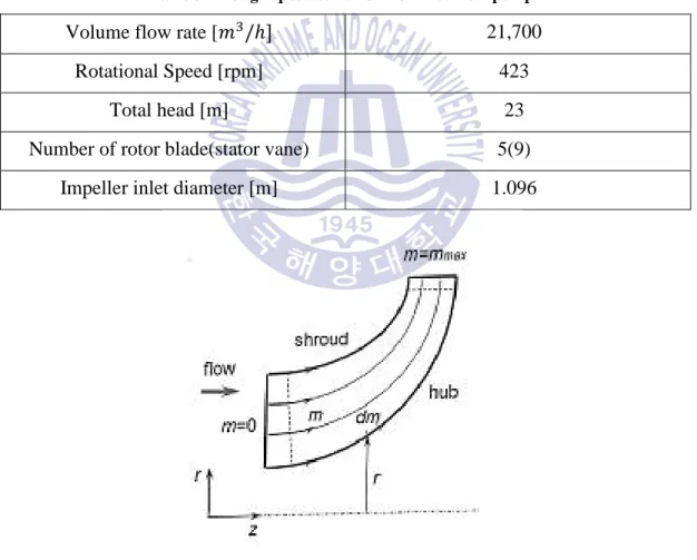
Table 3.1 shows the design specifications of mixed flow pump. The flow rate at the design point is 21700 /‘, the total head is 23 m, and the rotation speed is 423 rpm, the numbers of blades and diffusor 5 and 9 respectively. In multistage pump design, the definition of the meridian for the rotor and diffusor is required and has a great effect on pump efficiency. Fig. 3.3a shows the shape of meridian that is commonly using in fluid machinery design.

Table 3.1 Design specification of the mixed flow pump

Volume flow rate [ /‘g 21,700 Rotational Speed [rpm] 423

Total head [m] 23

Number of rotor blade(stator vane) 5(9) Impeller inlet diameter [m] 1.096

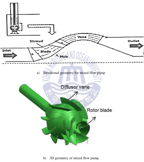
The blade profile of the mixed flow pump is created in bladeGen. Fig. 3.3b shows the 3D geometry of the mixed flow pump.

a) Meridional geometry for mixed flow pump

b) 3D geometry of mixed flow pump

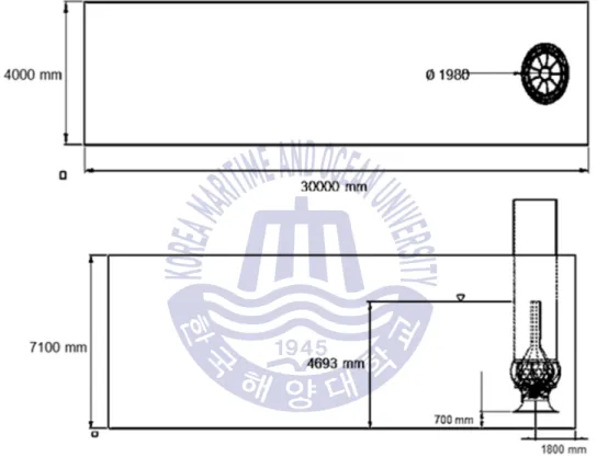
As illustrate in Fig.3.4, the total flow direction length of the model is 30m, the width and height of channel are 4.0m, 7.1m respectively. The center of the intake bell is located at 1.8m, 2.0m and 0.7m from rear wall, side wall and bottom, respectively. All the dimensions referred the recommended values in HI standard.

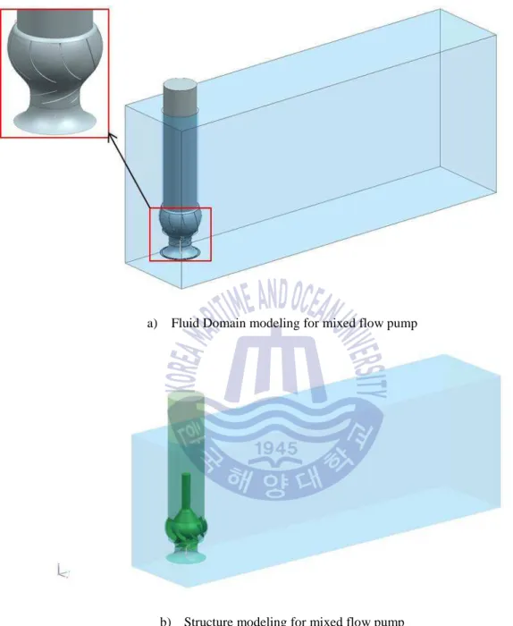
a) Fluid Domain modeling for mixed flow pump

b) Structure modeling for mixed flow pump

Mesh generation

ANSYS AIM enables you to mesh structural and fluids models. The primary tools for meshing are Meshing tasks and Volume Creation tasks.

To begin any study, we can set up a simulation process by launching a template that provides pre-set tasks and values for a given physics type, or can start a simulation process manually by importing and/or configuring geometry and then adding the desired tasks. Consider this information about which tasks to add if you are defining the simulation process manually. For structural simulations, or for fluid flow simulations where the flow volume has already been defined, add a Meshing task to mesh the output of the import or configuration task.

ANSYS AIM uses part-based meshing to mesh the entire part or assembly of parts in parallel. By default, it attempts to mesh sweepable bodies with hexahedrons and provides a tetrahedral mesh on bodies that are not sweepable or if the quality of the hexahedral mesh is poor. The mesh includes prism elements if inflation layers are generated. For other fluid flow simulations, add a Volume Creation task to:

• Define ("extract") a flow volume

• Group bodies into a single flow volume

• Simplify a body that has many surface patches

In this study ICEM CFD was used to generate the mesh of the sump fluid domain mixed flow pump domain.

consuming to build whereas hexahedral meshes provide more accurate results that the mesh quality is high.

The flow domain for two phase sump model was divided into a number of smaller region for two reasons. Firstly, it improved mesh quality and secondly it enabled named selection to be created. The mesh quality was improved by separating the floe domain in regions from complex geometrical shapes. Name selection were utilized to specify boundary conditions and to facilitate results viewing.

As the overall mesh shows, the scaled two phase sump model is divided into several parts to employ hexahedral mesh. The total nodes number is about 2.43 millions. Fig. 3.6 shows the overall mesh of sump domain as complex fluid domain was divided into 5 parts. The grid details of bell mouth and sump domain are shown in Fig. 3.7. Whereas Fig. 3.8 and Fig.3.9, show the mixed flow pump and sump top view grid generation. The mesh information of various parts is summarized in Table 3.2.

Table 3.2 Mesh information for impeller and diffuser

Item Number of nodes Mesh type Impeller domain 1,050,000 Tetra-Hedral Diffuser domain 1,400,000 Tetra-Hedral Inpart Domain 1,300,000 Tetra-Hedral

Fig. 3.8 Top view mesh generation

Fig. 3.9 Mixed flow pump mesh generation

Numerical approach

convergence result to predict the flow condition. The physics of the simulation domain was defined in CFX-Pre, the preprocessing module of ANSYS CFX.All simulation were performed using ANSYS CFX with HP MPI Distributed Parallel model.

A free surface is an interface between a liquid and a gas in which the gas can only apply a pressure on the liquid. Free surfaces are generally excellent approximations when the ratio of liquid to gas densities is large. Most CFD codes include the volume of fluid (VOF) technique, which was originally developed by Hirt and Nichols[24].

In our study, for the two phase model, both the phases (air and water) were distinctly defined by giving initial volume fraction as either Zero or one. Initial free surface was the separation of the sump water domain and air domain. The top of air domain is assigned as opening condition with equal to atmospheric pressure. Buoyant reference density of air is assigned to all domains.VOF is used to model the interaction between the two phases. The table shows the CFX pre setup parameter for two phase model.

For the full size pump sump model, the sump and stator fluid domain are stationary components while pump rotor is the rotating component. As for a boundary condition, the total pressure was specified at the inflow boundary, whereas the mass flow rate was specified at the outlet section of the pump stage. All computations have been carried out using water at 25° C as a working fluid. All the outer walls of the flow region and the internals walls were specified as the boundary type wall with flow condition as no slip. The ANSYS CFX-solver was

used to obtain the solution of the CFD problem. The solver control parameters were specified in the form of solution scheme and convergence criteria .High resolution was specified for the solution while for convergence the residual target for RMS values was specified as 1 “ 10A .

For the cavitation phenomena study, the working fluid is changed to two phases (water and water vapor at 25° C). Rayleigh Plesset model is selected for the cavitation model and the required parameters, Saturation pressure is set to the value of 3574 Pa, and the mean nucleation site diameter is specified as the default value of 2.0IA” m. The initial condition in fluid setting should use water volume fraction of 1 and water vapor volume fraction of 0.

Experimental setup

The experimental setup carried out in Korea Maritime and Ocean University, as shown in Fig. 3.10 the water is circulated through one channel with the help of 55kW pump. An inverter is applied to control the pump rpm and hence the mass flow rate. A four blade zero-pitch swirl meter, which is supported by a low friction bearing, installed at about four suction pipe diameter (d) downstream from the pump suction to measure swirl angle of pump approaching flow. For the swirl meter, the tip to tip blade diameter is 0.75d and the length in flow direction is 0.6 and one of the four blades is painted yellow as a reference to count revolution. The swirl angle analysis and vortices prediction checked for each case and as flow swirl usually un steady the observation time of swirl meter should be a continuous period of time comparison together. As show in Table 3.3, five cases have been studied,

the cases sequence started from the maximum flow rate 153.5 /‘ and, afterward the flow was decreased to minimum value 30.7 /‘ .

Table 3.3 Study cases

Case No Flow rate ( /‘)

Case 1 153.5

Case 2 30.7

Case 3 61.4

Case 4 92.1

Case 5 122.8

The experimental test details carried out by the following operation procedure: 1) Before start, all instruments have been checked out, calibrated and found ready to use.

2) Pump sump have been inspected for cleanliness and confirming to the the design specification.

3) Fill slowly the pump intake with clean waters slightly until the standard water level by adjusting the valve in the water supply line.

4) Supply clean water to the priming line.

5) Before running the pump, ensure that no air in the pump by open ventilation valve on pump casing.

6) Run the pump sump with the control valve in the pipe line closed 7) Set the required capacity by adjusting the control valve.

8) Chang the capacity by inverter and repeat steps 2 to 5. Measuring Instruments

1) Flow Meter (Electro-magnetic Flow Meter)

• Maker: Korea Flowmeter Company.

• Model No : KTM-900

• Range of current: From 0.3m/s to 10m/s

2) Control Valve

• Maker :joying, Korea

• Valve type: Ball Valve

• Ball Material : Plastic

• Operation: Manual

3) Pump

• Type : Centrifugal

• Maker: Hyosung Goodsprings, INC.

• Capacity: 550m^3/h

• Head : 18m

• Motor Power :45 KW 4) Inverter

5) Swirl Meter

• Maker : Shinhan Precision, Korea

• Blade No : 4 flat Blade

• Material : Stainless steel

Swirl angle analysis

The Swirl angle predicts the intensity of the flow rotation, and considers an important parameter to determine the quality of flow ingested by sump. The Hydraulic institute prescribes the method that needs to be employed for estimating this parameter. High Swirl in the pump intake can cause significant change in the operation conditions for a pump, and effects on the flow capacity, power requirement and efficiency. The instrumentation prescribed by ANSI/HI 9.8-2012 for measure the swirl angle is swirl meter.

Swirl meter rotation

The swirl meter in our study represent by rigid body as free rotation around Z axis, which all the particles of the body except rotation along circular bath. General when a body is rotating about a fixed axis, any point P located in the body travels along a circular bath. The motion of the body is described by angular motion which involves three basic quantities: angular position (θ ), angular velocity (n) and angular acceleration (q), described as follows [21] :

Fig. 4.1 Angular Motion [21]

• Angular Velocity. If • is the angular position of a radial line r located in some representative plane of the body, the angular velocity n has magnitude as n 5–

5N; direction along the axis of rotation and sense of direction either

clockwise or counterclock wise.

• Angular Acceleration. The angular acceleration q has magnitude q =5r_5N =

5`_–

5N`; its sense of direction depends on whether n is increasing or decreasing. In next chapter more details will explain about CFD analysis for Swirl meter rotation method.

Swirl angle method

Fig. 4.2 depicts the schematic view of the swirl meter and its installation, a four blade zero-pitch swirl meter, which is supported by a low friction bearing, will be installed at about four suction pipe diameter (d) down from the pump suction to measure swirl angle of pump approaching flow. For the swirl meter, the blade length in flow direction is 0.6d, the tip to tip blade diameter is 0.75d. One of the four blades is painted yellow as a reference to count revolution. As flow swirl is usually unsteady, the observation time of swirl meter reading should be a continuous period of time.

(4.1) (4.2) (4.3)

Where:

θ

V

: flow rotation speed at swirl meter (m/s).

Vz

: Average axial velocity at swirl meter (m/s). n: revolution per minute (rpm)

d: Diameter of pipe at swirl meter(m) Q: flow rate ( /s)

For the swirl angle calculating method by CFD, the key point is to obtain the average tangential velocity, so the swirl check circle were created as illustrate in Fig. 4.3. The swirl check circle is located at the section of 4d height with diameter of 0.25d, 0.5d and 0.75d respectively. z

V

V

_θ

θ

1

tan

−

=

2

4

d

Q

Vz

π

=

60

dn

V

_θ

=

π

Fig. 4.3 Schematic view of swirl angle numerical calculation

(4.4) Where:

θ

V

: Average tangential velocity (m/s)

V: circumferential velocity of check point in check circle, respectively (m/s) N: check point total numbers in single check circle

Rigid body motion

In our study the swirl meter set in CFX pre setup as a rigid body with free rotation about Z axis with 2 degree of freedom (2DOF) and no translation movement. In general, ANSYS CFX computes the position and orientation of a rigid body using

2

3

/

/

/

₁ 0.5 ₁ 0.75 1 0.25

+

+

×

=

∑

∑

∑

N N i i N i

N

V

N

V

N

V

V

_θ

equations of motion. These equations can provide up to six degrees of freedom (6 DOF), up to three translational and up to three rotational degrees of freedom.

In the context of rigid bodies in ANSYS CFX, an orientation is represented by a collection of three Euler angles that follow the ZYX convention. Under this convention, a reference coordinate frame is reoriented so that it acquires the orientation of interest as follows [22]:

•Euler Angle Z modifies the initial orientation by a rotation about the Z axis (using the right-hand rule to determine the direction).

•Euler Angle Y then further modifies the orientation by a rotation about the (modified) Y axis (using the right-hand rule to determine the direction). •Euler Angle X then further modifies the orientation by a rotation about the

(twice modified) X axis (using the right-hand rule to determine the direction).

Fig. 4.4, shown the same rigid body after being reoriented. The mounting system has pairs of pins at each pivot location. The angle that develops between a pair of pins at a given pivot is the Euler angle associated with the axis on which the pivot was initially located.

Fig. 4.4 Rigid body reoriented with Euler

Swirl angle results

As mentioned in chapter, swirl angle is predicting the intensity of flow rotation. Table 4.1 shows the swirl angle results both in CFD and experiment .for experiment the rotation of swirl meter is recorded over 10 minutes .As shown in Fig. 4.5, the two ways used to estimate the swirl angle by CFD method showed good agreement with an experimental result. Fig. 4.6 shows tangential velocity profile for each case. If we analyze one of these cases we find that minimum value for average velocity occurs at 0.25d and 0.75d because of the no slip condition and

the maximum value at the center of swirl meter at 0.5d. Also the higher expected fluctuation for tangential velocity indicates good agreement with high swirl angle

Table 4.1 Swirl angle results Case No Pump operation (m3h−1) Average Velocity (ms−1)

Swirl angle results Experimental (deg) CFD rigid body (deg) CFD circles check(deg) Case 1 153.5 0.48 18 18.3 19.1 Case 2 30.7 0.07 15.5 13.1 14 Case 3 61.4 0.12 15.9 15.3 16.9 Case 4 92.1 0.23 17.2 16.2 15.8 Case 5 122.8 0.35 18.1 19 17.5

CFD Rigid body * : This way used to find the swirl angle depend on swirl meter rotation (swirl meter setup as rigid body) ,its available directly by monitor the change in Euler angle with time step in CFX solver.

CFD tangential velocity *: the details of this method in section 4.2 (equation 4.4).

Results and Discussion

In this section two model cases results will be discussed. First case is vortices prediction (free surface vortex, submerged and side wall vortex) in details, by location, occurrences and air entrance. In second results, hydraulic performances of the mixed flow pump for head rise, shaft power, and pump efficiency versus different flow rate studied by performances curve with and without sump.

Vortices Results Free surface vortex

By the experimental test and CFD the four type of free vortex have been observed as shown in Fig. 5.1, the way free surface vorticity was observed by CFD depends on specifying different air volume fraction for each type. It was observed that 0.001-0.005 was a good range to observe free surface vortex. The first stage of vortex formation which was observed at 0.005 air volume fraction. The flow behaves as a constant swirl of surface and very small deformation of surface curvature. Type 2 shows surface dimple and deformation and this type was observed at 0.002 air volume fraction value. In types 5 and 6 air entrainment starts to occur and pull air bubbles under the liquid surface and enters together with liquid via the hole up to the bell mouth. The minimum air volume fraction was observed at these cases. Generally the free surface vortex is unsteady behavior with various locations and duration.