1. INTRODUCTION
Cranes are widely used to transport cargo (payloads) from one place to another in various areas: ports, warehouses, factories, construction sites, etc. During the previous two decades, the endeavor to enhance the handling efficiency of loads in industry as well as at ports has pulled vigorous research in two directions: one is the fast movement of loads between two places. Cranes can be categorized into four types: container cranes, overhead cranes, tower cranes, and jib cranes. In this paper, we are focusing on the container cranes that transport containers between a container-ship and trucks or automated guided vehicle in a container terminal.
In this paper, an energy-based (Lyapunov-function-based) nonlinear control design for a container crane is investigated. The advantage of using an energy-based control is that the nonlinearity of the plant can be fully incorporated into control law design when the energy function is differentiated along the plant dynamics. Also, the uniform asymptotic stability of the closed-loop system can be guaranteed by a properly chosen Lyapunov function. However, the disadvantage of energy-based control is that it is difficult to improve the transient performance (i.e., rise time, settling time, etc.) in a systematic way even though its stability is assured. Hence, a trial and error approach to improve the transient performance is normally pursued.
The contributions of this paper are the following. An axially moving nonlinear string model for container cranes is firstly derived. As control input, the use of an AMD system beside the gantry input is proposed. A boundary control law that utilizes the gantry velocity, the payload velocity, and the slope of the rope at the gantry position is derived. The uniform asymptotic stability of the closed-loop system is assured. Finally, the developed algorithm is verified through experiments using a pilot crane.
2. EQUATIONS OF MOTION
2.1 System Modeling
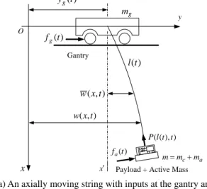
Fig. 1a shows a schematic diagram of the container crane modeled as a flexible cable system. It is assumed that the rope is inextensible and its dynamics can be modeled as a translating (axially moving) string equation. It is also assumed that the sway motion of both the load and rope occurs in a two-dimensional vertical plane. The transversal (lateral)
displacement of the rope from the gantry’s x-axis is relatively small compared with the displacement of the gantry itself.
Let t be the time, x be the spatial coordinate in the x-axis, that is, along the longitudinal direction of the rope, ρ be the mass per unit length of the rope, and l(t) be the length of the rope, which changes in time. Let yg(t) be the displacement of the gantry. Let w( tx, ) be the displacement
y
Payload + Active Mass
) (t yg ) (t fg Gantry ) (t fa a c m m m= + g m ) (t l ) , ( tx w ) , ( tx w x x′ O ) ), ( (lt t P
(a) An axially moving string with inputs at the gantry and/or payload positions. a m k c m a f a y a f
c
) ), ( ( tan−1wxlt t = θ(b) The inclined payload.
Fig. 1 Model as an axially moving string system with control inputs at both boundaries.
Sway Control of Container Cranes as an Axially Moving Nonlinear String
Hahn Park* and Keum-Shik Hong
*** Department of Mechanical and Intelligent Systems Engineering, Pusan National University, Busan, Korea (Tel : +82-51-510-1481; E-mail: [email protected])
**School of Mechanical Engineering, Pusan National University, Busan, Korea (Tel : +82-51-510-2454; E-mail: [email protected])
Abstract: The control objectives in this paper are to move the gantry of a container crane to its target position and to suppress the transverse vibration of the payload. The crane system is modeled as an axially moving nonlinear string equation, in which control inputs are applied at both ends, through the gantry and the payload. The dynamics of the moving string are derived using Hamilton’s principle. The Lyapunov function method is used in deriving a boundary control law, in which the Lyapunov function candidate is introduced from the total mechanical energy of the system. The performance of the proposed control law is compared with other two control algorithms available in the literature. Experimental results are given.
Keywords: Container crane control, nonlinear string equation, boundary control, sway suppression, transverse vibration, partial differential equation, Hamilton’s principle, Lyapunov method.
of the rope from the vertical axis, x′ in Fig. 1a, at spatial coordinate x and time t . Let P( tx, ) be the tension of the rope caused by the weights of the payload and the cable itself. Therefore, the displacement w( tx,), velocity, and acceleration of the rope at x and t are given by
) , ( ) ( ) , (xt y t w xt w = g + , (1a) x t g g w l w t y Dt t x w D Dt t y D Dt t x w D & & + + = + = () ( , ) () ) , ( , (1b) w l w l w l w t y Dt t x w D x xt tt g 2 2 2 2 ) ( ) ,
( & && &
&& + + + +
= , (1c)
where in above equation
( )
⋅t=∂( )
⋅/∂t and( )
⋅x=∂( )
⋅ /∂x denote the partial derivatives in t and x , respectively, andx l t Dt
D(⋅)/ =∂(⋅)/∂ +&∂(⋅)/∂ is the material derivative (see Munson et al. (2002) for its definition) due to the axial transport phenomenon of the cable while hoisting of the rope, in which l& is the up-down velocity of the rope. Note that if a variable is a function of time only, then ( &⋅ is used instead of ) the partial derivative notation, for example, l&(t), )y&g(t , etc. Note also that the gantry position has nothing to do with the spatial coordinate, the following relationship hold:
xx xx x
x w w w
w = . and = (2)
2.2 Active Mass-Damper System
In Fig. 1a, let m , g m , and c m be the mass of the a gantry, the payload, and the actuator (AMD system), respectively. Let fg(t) and fa(t) be the control force applied at the gantry and the payload, respectively. The AMD system is widely used in civil engineering, for example, in suppressing the structural vibration of a tall building. In that case, a huge mass can be used to generate a large control force. But, in our case because the active-mass should move on top of the spreader, its size is limited. Consequently, the control force is limited. Therefore, it would be desirable to use the gantry force to suppress a large sway angle and use the AMD force to suppress the residual sway motion that remains at the end of a gantry stroke.
In Fig. 1b, the inclined spreader is depicted. Let y be the a
displacement of the active-mass from its neural position. If the spreader is pulled by a single rope and the connection between the rope and the spreader is a pin joint, the inclination angle of the spreader can be described independently with the slope of the rope at its end point. However, in actual cranes, the spreader is normally pulled by at least four ropes. Therefore, the inclination, θ , of the spreader can be derived as a function of the slope of the rope at the end point as follow:
(
lt t)
wx (),
tan−1 =
θ . (3)
As the spreader swings, the tension increase in the rope due to the active-mass changes from mag to magcosθ, whereas a reversal force to the motion of the active-mass is generated as much as magsinθ . The equation of motion of the active-mass is given by a a a a a ay cy ky m g f
m && + & + + sinθ= , (4)
where c and k are the damping coefficient and the spring constant of the AMD system. Equation (4) provides an idea how large control force can be generated using ma, c, and k. Now, the tension generated due to the payload and the AMD system becomes
(
)
(
m m lt x)
t x P( , )= ( c+ a)+ρ ( )−(
)
(
gcostan 1wx(x,t) −l(t))
− fasinθ× − &&
. (5)
In reality, the mass of the payload together with the spreader is much larger than that of the active-mass, which justifies the negligence of the second term in the right-hand side of (5). Also, by assuming that the sway angle is relatively small, the following simple form of the tension along the rope is used in this paper (Zhu and Ni, 2000; Zhu et al., 2001).
(
)
(
( ) ())
(
())
) , (xt m m lt x g l t P ≅ c+ a +ρ − − && . (6) 2.3 Equations of MotionNow, to derive the equations of motion, the following extended Hamilton’s principle (Rahn et. al., 1999; Zhu and Ni, 2000).
(
)
0 2 1 = + −∫
t T V W dt t δ δ δ , (7)where T is the kinetic energy, V is the potential energy (the strain energy of the rope), and Wδ is the virtual work done by the forces fg(t) and fa(t).
The kinetic energy of the gantry, the rope, and the payload is
∫
⎪⎭ ⎪ ⎬ ⎫ ⎪⎩ ⎪ ⎨ ⎧ ⎟⎟ ⎠ ⎞ ⎜⎜ ⎝ ⎛ + + ⎟⎟ ⎠ ⎞ ⎜⎜ ⎝ ⎛ = () 0 2 2 2 2 1 ) , 0 ( 2 1 lt g dx t D w D l t D t w D m T ρ & ⎪⎭ ⎪ ⎬ ⎫ ⎪⎩ ⎪ ⎨ ⎧ ⎟⎟ ⎠ ⎞ ⎜⎜ ⎝ ⎛ + + 2 2 ((), ) 2 1 t D t t l w D l m &. (8)
Note that (8) includes the translational kinetic energy of the rope due to hoisting (i.e., l& terms) as well as the transversal 2 kinetic energy of the rope (i.e., (Dw/Dt)2 terms). The potential energy is
∫
⎟ ⎠ ⎞ ⎜ ⎝ ⎛ + = () 0 2 2 ) , ( t l x x dx EA t x P V ε ε∫
⎟ ⎠ ⎞ ⎜ ⎝ ⎛ + = () 0 2 2 4 ) , ( 2 1 lt x x w dx EA w t x P . (9)where εx is the strain of the rope. The second equality in (9) has been derived from the view point that if the infinitesimal distance dx is replaced by the infinitesimal length ds , the strain εx can be approximated as (Wickert, 1992)
2 2 1 x x≅ w ε . (10)
The virtual works done by fg(t) and fa(t) are ) ), ( ( ) ( ) , 0 ( ) (t w t f t wlt t f W g δ a δ δ = + . (11)
Because the rope length l(t) changes with time, the domain of integration for the spatial variable x is time-dependent. Thus, the standard procedure for integration by part with respect to the temporal variable does not apply. The use of Leibniz’s integral rule, for instance, gives
∫
⎟ ⎠ ⎞ ⎜ ⎝ ⎛ ∂ ∂ () 0 t l wdx Dt Dw t ρ δ ) ( ) ( 0 ) ( 0 t l x t l t l t w Dt Dw l wdx Dt Dw t dx w Dt Dw = ⎥ ⎦ ⎤ ⎢ ⎣ ⎡ ⎟ ⎠ ⎞ ⎜ ⎝ ⎛ − ⎟ ⎠ ⎞ ⎜ ⎝ ⎛ ∂ ∂ + ⎟ ⎠ ⎞ ⎜ ⎝ ⎛ =∫
ρ δ∫
ρ δ & ρ δ . (12)Note that the above equation is used to calculate the variation of kinetic energy of rope.
Following the general procedure for integration by parts with respect to the spatial variable and integrating (12) from
1
t to t2, imposing vanishing variations of δw at t1 and
2
t , the result of (7) becomes
[
]
wdxdt Dt w D w EAw x w t x P t t t l xx xx
ρ δ∫ ∫
⎪⎭ ⎪ ⎬ ⎫ ⎪⎩ ⎪ ⎨ ⎧ ⎟ ⎟ ⎠ ⎞ ⎜ ⎜ ⎝ ⎛ − + 2 2 ) ( 0 2 2 2 2 3 ) , ( dt w Dt w D m Dt Dw l EAw w t x P t f x g t t g x x 0 2 2 3 2 1 2 1 ) , ( ) ( = ⎪⎭ ⎪ ⎬ ⎫ ⎟ ⎟ ⎠ ⎞ ⎜ ⎜ ⎝ ⎛ − ⎩ ⎨ ⎧ ⎟⎟ ⎠ ⎞ ⎜⎜ ⎝ ⎛ − + + +∫
ρ& δ0
)
(
2
1
)
,
(
) ( 2 2 3 2 1=
⎪⎭
⎪
⎬
⎫
⎪⎩
⎪
⎨
⎧
+
⎟
⎟
⎠
⎞
⎜
⎜
⎝
⎛
−
−
−
+
=∫
f
t
w
dt
t
D
w
D
m
EAw
t
x
P
t l x t t x aδ
.(13)Setting the coefficient of wδ to zero in (13) yields the governing equations as 0 2 3 ) ) , ( ( 2 2 2 = − − ⎟ ⎟ ⎠ ⎞ ⎜ ⎜ ⎝ ⎛ xx x x x EAw w w t x P Dt w D ρ , 0<x<l(t), (14a) or 0 2 3 ) ( ) 2
(wtt+ l&wxt+l&&wx+l&2wxx −Pwx x− EAwx2wxx=
ρ ,
) (
0<x<lt , (14b) and the boundary conditions are
)
(
2
1
)
,
(
3 2 2t
f
EAw
w
t
x
P
Dt
Dw
l
Dt
w
D
m
g⎟
−
x−
x=
g⎠
⎞
⎜
⎝
⎛
+
⎟
⎟
⎠
⎞
⎜
⎜
⎝
⎛
&
ρ
, at x=0, (15a))
(
2
1
)
,
(
3 2 2t
f
EAw
w
t
x
P
Dt
w
D
m
⎟
⎟
+
x+
x=
a⎠
⎞
⎜
⎜
⎝
⎛
, at x=l(t). (15b) Note that (15a,b) represent dynamical features of the gantry and the payload. It is remarked that if we consider the linear string (i.e., neglect the term related with EA) andl&=0,Dt
Dw / is equal to wt and D2w/ Dt2 is equal to wtt.
Finally, it is observed that by setting l&=0, 0EA= , and 0
) (t =
fa , the resulting equations of (14)-(15a,b) coincide
with those in Rahn et al. (1999).
3. CONTROL LAW DESIGN
The control objectives in this paper are, firstly, to regulate (move) the gantry at a target position and, secondly, to suppress the payload vibration when the gantry reaches its target position. For this, we adopt the Lyapunov function method, which yields the uniform asymptotic stability of the closed-loop system with a properly chosen Lyapunov function. For notational convenience, we use P , w , and l , by omitting the independent variables x and t , in place of
) , ( tx
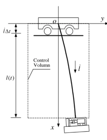
P , )w( tx, , and l(t). The control volume at time t, as shown in Fig. 2, is defined as the spatial domain 0≤x≤l(t).
Recalling that the plant in this paper consists of the axially translating rope, the gantry, and the payload (including the active-mass), the total mechanical energy of the system at time t is given by ) ( ) ( ) (t E t E t Esystem = rope + g+p , (16) where y l& t l&∆ ) (t l x o Control Volumn
Fig. 2 The control volume of the axially moving rope with variable length. ) ( ) (t E t Erope = cv dx w EA w P Dt Dw l t l x x
∫
⎥⎥ ⎦ ⎤ ⎢ ⎢ ⎣ ⎡ + + ⎟ ⎠ ⎞ ⎜ ⎝ ⎛ + = () 0 4 2 2 2 8 2 1 2 1 2 1ρ& ρ∫
= () 0 ( , ) t l dx t x ε,
(17) 4 2 2 2 8 2 1 2 1 2 1 ) , ( Pwx EAwx Dt Dw l t x ⎟ + + ⎠ ⎞ ⎜ ⎝ ⎛ + = ρ ρ ε & , (18) and ⎪⎭ ⎪ ⎬ ⎫ ⎪⎩ ⎪ ⎨ ⎧ ⎟ ⎠ ⎞ ⎜ ⎝ ⎛ + + ⎟ ⎠ ⎞ ⎜ ⎝ ⎛ = + 2 2 2 ) ), ( ( 2 1 ) , 0 ( 2 1 ) ( Dt t t l Dw l m Dt t Dw m t Eg p g & .(19) ) (tErope and Eg+p(t) represent the mechanical energy of
the rope and that of the gantry and payload at time t , respectively. Ecv(t) denotes the mechanical energy of the rope in the control volume and, therefore, Erope(t)=Ecv(t) at time t . In (18), ε( tx, ) denotes the mechanical energy of the rope per unit length (i.e., energy density), in which
2 /
2
l&
ρ and
(
ρ(
Dw/Dt)
2+Pwx2+EAwx4/4)
/2 represent the energy density associated with the rigid-body translation and the transverse vibration of the rope, respectively. The two terms in the right-hand side of (19) denote the kinetic energy of the gantry and that of the payload including the active-mass, respectively.Remark 1: The differentiation of Ecv(t), using Leibnitz’s rule, yields:
(
lt t)
l dx t t x t Ecv() l(t) ( , ) (), 0 ε ε & & + ∂ ∂ =∫
. (20) ) (tE&cv describes the instantaneous growth and decay of total mechanical energy of the translating rope with variable length. Because the translating medium gains and loses mass during lowering (l&>0) and lifting (l&<0), respectively, Ecv(t) increases and decreases accordingly. Even though the total mechanical energy involves the energy of the longitudinal motion, the stability analysis of the control algorithm for suppressing the transverse vibration can be done by omitting the energy in the longitudinal direction.
At time t+∆t, the control volume becomes the spatial domain [0,l(t)+ &l∆t], and the material particles of the rope has translated a distance l& . At time ∆t t+∆t, the mechanical energy of the particles occupying the spatial domain [l&∆t,l(t)+l&∆t] becomes (Zhu, 2002, equation (26))
) , 0 ( ) ( ) (t t E t t l t t t Erope +∆ = cv +∆ −&∆ ε +∆ . (21)
Therefore, by sending ∆t→0 , the rate of change of ) (t Erope becomes ) , 0 ( ) (t E l t
E&rope = &cv−&ε , (22)
which results in the Reynolds transport theorem for a translating medium with variable length (Zhu and Ni, 2000).
Now, based upon (16) and Remark 1 (for suppressing the transverse vibration, the rigid-body translational motion of the rope can be omitted for the stability analysis of the closed-loop system), a Lyapunov function candidate for the purpose of suppressing the transverse vibration and regulating the gantry target position is considered as follows:
) ( ) ( ) (t V1t V2 t V = + , (23) where dx w EA w P Dt Dw t V
∫
lt x x ⎥ ⎥ ⎦ ⎤ ⎢ ⎢ ⎣ ⎡ + + ⎟ ⎠ ⎞ ⎜ ⎝ ⎛ = () 0 4 2 2 1 2 8 1 2 1 ) ( ρ , (23a) 2 2 2 ) ), ( ( 2 1 ) , 0 ( 1 1 2 1 ) ( ⎟ ⎠ ⎞ ⎜ ⎝ ⎛ + ⎟ ⎠ ⎞ ⎜ ⎝ ⎛ ⎟⎟ ⎠ ⎞ ⎜⎜ ⎝ ⎛ + = Dt t t l Dw m Dt t Dw m K t V g a{
(0, )}
2 1 1 2 1 d p a w t w K K ⎟⎟⎠ − ⎞ ⎜⎜ ⎝ ⎛ + + , (23b)where Ka and Kp are the control gains. Now, the time-derivative of (23) is evaluated by (20) and applying the definition of material derivative to V2(t).
First, ∂ε(x,t)/∂t is calculated as follow:
⎭ ⎬ ⎫ ⎩ ⎨ ⎧ + + + ∂ ∂ = ∂ ∂ 2 2 4 8 2 1 ) ( 2 1 ) , ( x x x t w EA w P w l w t t t x ρ & ε
{ }
( ) ( ) 2 3 )(wt l&wx Pwx x EAwx2wxx⎟− wt+l&wx l&wxt+l&2wxx ⎠ ⎞ ⎜ ⎝ ⎛ + + = ρ xt x xt x x tw Pw w EAw w P 2 3 2 1 2 1 + + +
. (24)
Using (24), (22) is given by[
]
() 0 ) ( 0 ( , ) ( , ) t l t l t x l dx t x tε ε & + ∂ ∂∫
∫
+ ⎥ ⎥ ⎦ ⎤ ⎢ ⎢ ⎣ ⎡ ⎟⎟ ⎠ ⎞ ⎜⎜ ⎝ ⎛ ⎟ ⎠ ⎞ ⎜ ⎝ ⎛ + = () 0 2 ) ( 0 3 2 1 2 1 lt x t l x x w dx t D DP t D w D EAw Pw . (25)The material derivative of the tension,DP /Dt, is )} ) ( ( {m lt x l P l P t D DP x t+ =− + −
= & &&& ρ . (26)
The substitution of (26) into (25) yields: ) ( 0 3 2 1 lt x x rope t D w D EAw Pw Dt DE ⎥ ⎥ ⎦ ⎤ ⎢ ⎢ ⎣ ⎡ ⎟⎟ ⎠ ⎞ ⎜⎜ ⎝ ⎛ ⎟ ⎠ ⎞ ⎜ ⎝ ⎛ + =
∫
+ − − () 0 2 )} ) ( ( { 2 t l x dx w x t l m l&& ρ &.
(27)Next, the material derivative of V2(t), by applying the boundary condition (15a,b) is given by
3 2 2 1 ) ( 1 1 x x g a EAw Pw t D w D l t f t D w D K t D DV + ⎪⎩ ⎪ ⎨ ⎧ + ⎟⎟ ⎠ ⎞ ⎜⎜ ⎝ ⎛ − ⎟⎟ ⎠ ⎞ ⎜⎜ ⎝ ⎛ + = ρ&
{
}
}
) ( 3 0 2 1 ) ( ) , 0 ( t l x x x a x d p f t Pw EAw t D w D w t w K = = ⎭⎬ ⎫ ⎩ ⎨ ⎧ − − ⎟⎟ ⎠ ⎞ ⎜⎜ ⎝ ⎛ + − + . (28) Using (27) and (28), DV /Dt is∫
+ − − = () 0 2 )} ) ( ( { 2 t l x dx w x t l m l Dt DV &&& ρ 0 3 2 1 ) ( ) ( 1 1 = ⎪⎭ ⎪ ⎬ ⎫ ⎪⎩ ⎪ ⎨ ⎧ ⎟ ⎠ ⎞ ⎜ ⎝ ⎛ + − − + ⎟⎟ ⎠ ⎞ ⎜⎜ ⎝ ⎛ − ⎟⎟ ⎠ ⎞ ⎜⎜ ⎝ ⎛ + + x x x a d p g a EAw Pw K w w K t D w D l t f t D w D K ρ& ) ( ) ( t l x a Dt Dw t f = ⎟ ⎠ ⎞ ⎜ ⎝ ⎛ + . (29)Note that a positive and negative jerk l&&& generates a stabilizing and destabilizing effect. However, the stabilizing effect from a positive jerk is generally not sufficiently large to suppress the inherent destabilizing effect (Zhu and Ni, 2000). So we can neglect the first term on the right-hand side of (29).
The following feedback control law will make (29) negative semi-definite.
{
}
⎟⎟ ⎠ ⎞ ⎜⎜ ⎝ ⎛ − + − − = t D t w D K l w t w K t fg() p (0,) d (ρ
& dg) (0,) ⎟ ⎠ ⎞ ⎜ ⎝ ⎛ + + (0, ) 2 1 ) , 0 ( ) , 0 ( tw t EAw3 t P Ka x x , (30a) ⎟⎟ ⎠ ⎞ ⎜⎜ ⎝ ⎛ − = t D t t l w D K t fa da ) ), ( ( ) ( , (30b)where Kp,Kdg,Ka and Kda are positive constants. That
is, by (30a,b), (29) is given as follow:
0 ) ), ( ( ) , 0 ( 1 2 2 ≤ ⎟⎟ ⎠ ⎞ ⎜⎜ ⎝ ⎛ − ⎟⎟ ⎠ ⎞ ⎜⎜ ⎝ ⎛ + − = t D t t l Dw K t D t Dw K K t D DV da a dg . (31) Note that if we set l&=0, the material derivative has no meaning. And if we consider the rope as the linear string (i.e., neglect the term related with EA), then the control law in the case of a constant rope length becomes the following.
{
(0, )}
{
(0,)}
) (t K w t w K w t fg =− p − d − dg t ) , 0 ( ) 0 ( w t P Ka x + , (32a){
(
(
),
)
}
)
(
t
K
w
l
t
t
f
a=
−
da t . (32b)And if we set fa(t)=0, then (32a,b) are basically the same as the results of Rahn et al. (1999). The difference between (32a,b) and the results of Rahn et al.(1999) is caused by the difference of the Lyapunov function candidate and system characteristic (i.e, linear or nonlinear).
All the above developments are summarized in the following theorem.
Theorem: Consider the plant (14) and (15a,b). Then, the closed-loop system with the control law (30a,b) is uniformly asymptotically stable.
4. EXPERIMENTAL RESULTS
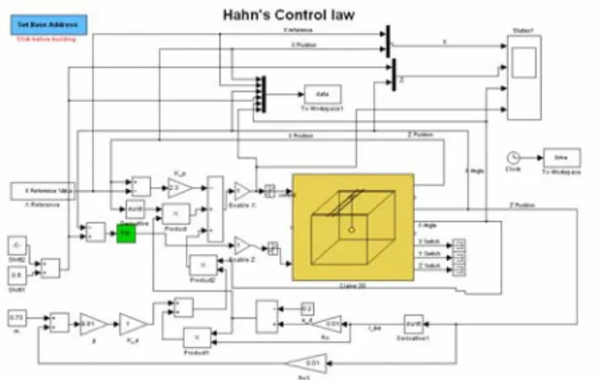
In this section, experimental results of the closed-loop system with the proposed control law (30a,b) are discussed. Fig. 3 shows the pilot crane used in experiment, which lacks the AMD system and, therefore, the responses of the closed-loop system with only the input to the gantry are discussed. In fig. 4, the controller for experiment is shown. It
Fig. 3 The 3-D pilot crane used in experiment: InTeCo 3DCrane (Poland).
Fig. 4 The controller for the experiment.
was constructed by Simulink. The material property of the rope and the payload mass, respectively, are ρ=0.01kg/m and m=0.73kg.
It is noted that Dw(0,t)/Dt in (30a) is given by ) , 0 ( ) ( ) , 0 ( ) , 0 ( ) ( ) , 0 ( t w l t y t w l t w t y t D t Dw x g x t
g & & &
& + + = +
= .
At the top end of the rope, the displacement w(0,t)=0 because the rope is attached to the gantry and, therefore,
0 ) , 0 ( t =
wt . For this reason, the applied control force is given
as a combination of the gantry velocity and the slope of the rope at the top end.
Using the same experimental conditions, experiments for the three control algorithms, in case of a constant rope length, were performed. Fig. 4 shows the sway angle of the E2 coupling control law of Fang et al. (2003), in which the used control gains are Kp=21, Kd=40, Ke=0.001, and Kv=46.
Fig. 5 compares the responses of the Rahn’s control law with 1
. 3 =
p
K , Kdg=1.3, and Ka=1 and those of the proposed control law (32a) with Kp=3.25, Kdg=1.2, and Ka=2.8. Comparing Fig. 4 and Fig. 5, a big improvement in sway suppression by using a PDE model is shown. Therefore, the control law design using a PDE model, rather than using an ODE model, is fully justified. However, observing Fig. 5, as far as the rope length is constant, there is not much improvement between the control law in Rahn et al. (1999) and the proposed one.
0 5 10 15 20 -0.2 -0.1 0.0 0.1 0.2 An gl e [ ra d ] Time [sec]
Fig. 4 Sway angle result of the E2 control law of Fang et al. (2003) (dotted lines: target values, solid lines:
experimental results). 0 5 10 15 20 -0.2 -0.1 0.0 0.1 0.2 An gl e [r ad ] Time [sec]
Fig. 5 Sway angle results of two control laws: Rahn et al. (1999)’s control law (1-dot chain line) and the proposed
control law (32a) (solid line)
0 5 10 15 20 -0.2 -0.1 0.0 0.1 0.2 A ngle [rad] Time [sec]
(a) Sway angle while extending the rope from 0.2 m to 1.0 m. 0 5 10 15 20 -0.2 -0.1 0.0 0.1 0.2 A ngle [ rad ] Time [sec]
(b) Sway angle while lifting-up the rope from 1.0 m to 0.2 m.
Fig. 6 Comparison of two control laws with changes of rope length (solid line: the proposed control law (30a), 1-dot
chain line: the control law of Rahn et al.(1999)) Fig. 6 compares the response of the Rahn’s control law, while changing the rope length from 0.2 m to 1.0 m and vice versa, and that of the proposed one (30a). An improvement with the use of (30a) is shown. This improvement will get
larger when l& gets larger. The used control gains, while lowering the payload, are Kp=2.3, Kdg=0.4, and Ka=2.5 and those gains, while lifting up the payload, are
4 . 9 = p
K , Kdg=5.7 and Ka=4.6. Finally, it is remarked that the proposed control law derived using a PDE model is much more effective in both suppressing the transverse vibration and also improving the rise time.
5. CONCLUSIONS
In this paper, we considered the anti-sway control problem of container cranes in the perspective of controlling an axially moving string system by applying control inputs at boundaries. Because the cranes are an underactuated mechanical system, the control input should be applied through dynamic coupling, that is, gantry motion. The main control input is normally given through the dynamics of the gantry motion, but for suppressing a small residual transverse vibration, an AMD can be effectively used.
ACKNOWLEDGMENTS
This work was supported by the Research Center for Logistics Information Technology, Pusan National University, funded by the Ministry of Education and Human Resources Development, Korea.
REFERENCES
[1] Y. Fang, W. E. Dixon, D. M. Dawson, and E. Zergeroglu, “Nonlinear coupling control laws for an underactuated overhead crane system,” IEEE/ASME Transactions on Mechatronics, Vol. 8, No. 3, pp. 418-423, 2003..
[2] Y. S. Kim, K. S. Hong, and S. K. Sul, “Anti-sway control of container cranes: inclinometer, observer, and state feedback,” International Journal of Control, Automation, and Systems, Vol. 2, No. 4, pp. 399-410, 2004.
[3] B. R. Munson, D. F. Young, and T. H. Okiishi, Fundamentals of Fluid Mechanics, John Wiley & Sons Inc., New York, 2002.
[4] C. D. Rahn, F. Zhang, S. Joshi, and D. M. Dawson, “Asymptotically stabilizing angle feedback for a flexible cable gantry crane,” ASME Transactions, Journal of Dynamic Systems, Measurement, and Control, Vol. 121, No. 3, pp. 563-566, 1999.
[5] J. A. Wickert, “Non-linear vibration of a traveling tensioned beam,” International Journal of Non-Linear Mechanics, Vol. 27, No. 3, pp. 503-506, 1992.
[6] K. J. Yang, K. S. Hong, and F. Matsuno, “Robust adaptive boundary control of an axially moving string under a spatiotemporally varying tension,” Journal of Sound and Vibration, Vol. 273, No. 4/5, pp. 1007-1029, 2004.
[7] W. D. Zhu and J. Ni, “Energetics and stability of translating media with an arbitrarily varying length,” ASME Journal of Vibration and Acoustics, Vol. 122, pp. 295-304, 2000.
[8] W. D. Zhu, “Control volume and system formulations for translating media and stationary media with moving boundaries,” Journal of Sound and Vibration, Vol. 254, No. 1, pp. 189-201, 2002.
[9] J. Y. Choi, K. S. Hong, and K. J. Yang, “Exponential Stabilization of an Axially Moving Tensioned Strip by Passive Damping and Boundary Control,” Journal of Vibration and Control, Vol. 10, pp. 661-682, 2004.
[10] K. S. Hong, C. W. Kim, and K. T. Hong, “Boundary Control of an Axially Moving Belt System in a Thin-Metal Production line,” International Journal of Control, Automation, and Systems, Vol. 2, No. 1, pp. 55-67, 2004