자동차
유동기인 실내소음 예측을 위한
CFD/FEM/BEM/SEA 의 조합 및 검증 – CAA German Working Group
Combining CFD/FEM/BEM/SEA to Predict Interior Vehicle Wind Noise –
Validation Case CAA German Working Group
D. Blanchet† ‡ , A. Golota*
Key Words : Wind Noise(유동소음), Convective & Acoustic Components(대류 및 음향 성분),
Aero-Vibro-Acoustics(유동-구조-음향), FEM(유한요소법), BEM(경계요소법), SEA(통계적 에너지 해석법), CFD(전산유체해석), Corcos Model(Corcos 모델), Wavenumber Transformation(파수 변환)
ABSTRACT
Recent developments in the prediction of the contribution of windnoise to the interior SPL have opened a realm of new possibilities in terms of i) how the convective and acoustic sources terms can be identified, ii) how the interaction between the source terms and the side glass can be described and finally iii) how the transfer path from the sources to the interior of the vehicle can be modelled. This work discusses in details these three aspects of wind noise simulation and recommends appropriate methods to deliver required results at the right time based on i) simulation and experimental data availability, ii) design stage at which a decision must be made and iii) time available to deliver these results. Several simulation methods are used to represent the physical phenomena involved such as CFD, FEM, BEM, FE/SEA Coupled and SEA. Furthermore, a 1D and 2D wavenumber transformation is used to extract key parameters such as the convective and the acoustic component of the turbulent flow from CFD and/or experimental data whenever available. This work focuses on the validation of the wind noise source characterization method and the vibro-acoustic models on which the wind noise sources are applied.
1. Introduction♣
In order to model wind noise it is necessary to understand the source, the paths which typically involve direct vibro-acoustic transmission through certain regions of the structure, transmission through nearby leaks/seals and isolation and absorption provided by the interior sound package and the receiver and in particular, the frequency range(s) in which wind noise provides an audible contribution to the interior noise in the occupant’ s ears. While many
† Corresponding Author; ESI Group
E-mail : [email protected] Tel : +49 89 4510888 14
‡ Presenter; ESI Group * ESI Group
regions of a vehicle can contribute to wind noise, the fluctuating surface pressures on the front side glass due to vortices and separated flow generated by the A-pillar and side mirror are often important contributors.
This paper presents an overview of different approaches that can be used to efficiently predict wind noise contribution to overall SPL at the driver’ s ear. After describing the physical phenomena involved in wind noise simulation, a review of major wind noise source characterization will be presented. Following is a description of vibro-acoustics methods used to predict interior SPL for a given wind noise source model. Finally, validation cases for both vibro-acoustics (VA) and Aero-Vibro-Acoustics (AVA) are presented.
2. From turbulent flow to vehicle interior SPL
2.1 Physical phenomena involved
A turbulent flow generated outside a vehicle contains both a convective and an acoustic pressure fluctuations component on side glass (Figure 1). This energy can potentially be transmitted to the interior of a vehicle and be detrimental to the sound quality or speech clarity experienced by occupants.
Figure 1. Turbulent flow generated behind side mirror and A-pillar
The following sections describe the main noise generation principles involved in wind noise.
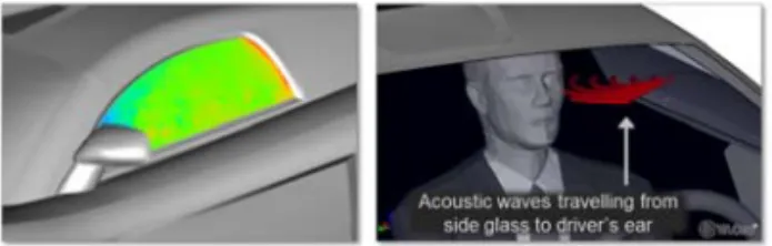
2.2 Pressure fluctuation on side glass The turbulent flow outside a vehicle generates a fluctuating surface pressure field on the side glass which includes a convective and an acoustic component. The convective component is related to the pressure field generated by eddies travelling at the convection speed. The acoustic component is related to acoustic waves travelling within the flow and being generated on various surfaces before reaching the side glass. The acoustic component is typically very small in amplitude compared to the convective component and as will be shown later in this paper, can be the major contributor at coincidence frequency of the side glass. Furthermore, the acoustic waves reaching the side glass are highly directional. Both the convective and the acoustic components contribute to the sound pressure level (SPL) at the driver‘s ear (Figure 2).
Figure 2. Fluctuating surface pressure on side glass (left) and acoustic waves propagating from side glass to the driver's ear
(right).
2.3 Pressure fluctuation on mirror
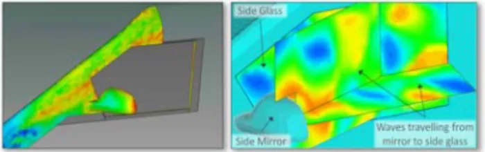
In Figure 3 on the left side, the pressure is the highest in the front of the side mirror. It is also the location of lowest fluctuation. The flow in front of the mirror is steady as opposed to the rear face of the mirror where the flow fluctuates the most. The turbulences at the rear face of the mirror create acoustic waves that travel rearward towards the side glass with a specific heading. This source term is associated to a dipole source (surface terms). The acoustic waves travelling towards the side glass are likely to be transmitted inside the vehicle through the side glass and to the driver’s ear as illustrated in Figure 3 on the right.
Figure 3. Fluctuating surface pressure on side mirror rear face (left) and acoustic waves propagating from
side mirror to the driver's ear (right) 2.4 Pressure fluctuation on A-Pillar
The same principle applies for the acoustic waves generated by turbulences in the vicinity of the A-Pillar. The acoustic waves travel to the side glass and are likely to be transmitted inside the vehicle to the driver’s ear (Figure 4).
Figure 4. Fluctuating surface pressure on A-Pillar (left) and acoustic waves propagating from A-Pillar to driver's ear
(right)
2.5 Acoustic sources within eddies
Eddies within the turbulent flow can also generate noise and therefore constitute acoustic sources. These sources act as quadrupole acoustic sources and are referred to as volume source terms. These acoustic sources are at close proximity to the side glass. At automobile speeds, these source terms are considered negligible (Figure 5).
Figure 5. Turbulent flow behind side mirror (left) and acoustic waves propagating from within turbulent flow to
the driver's ear (right). This contribution is negligible. 2.6 Pressure fluctuation on side glass – Outward effect
Pressure fluctuations on the side glass also generate acoustic waves that propagate away from the side glass. These waves can interfere with incoming acoustic waves from A-Pillar and mirror. It is believed to have a negligible impact on driver‘s ear SPL (Figure 6).
Figure 6. Fluctuating surface pressure on side glass (left) and acoustic waves travelling from side glass away from vehicle. The acoustic waves interfere with acoustic waves
coming from side mirror and A-Pillar (right). 3. Overview of available approaches
Several methods of representing wind noise sources have been investigated over the past 10
years in the automotive industry. Empirical methods have shown their merits and limitations especially when the geometry of the structure changes significantly compared to previous computations [1],[2],[3] and [4]. A more predictive approach, based on the ability of coupling time domain turbulent flow data to a vibro-acoustics model has opened new possibilities. The computation process is illustrated in Figure 7.
Figure 7. Illustration of source characterization (left) and vibro-acoustic modelling (right) approaches discussed in
this paper.
The left side of Figure 7 shows the source characterization topics that will be covered in the paper and the right side shows the vibro-acoustics methods that can be combined to compute the interior SPL. In this paper, the combination of an aero-acoustic (CAA) sources and a vibro-acoustic (VA) model is called an aero-vibro-acoustic (AVA) model.
3.1 Turbulent Flow Data
The turbulent flow can be represented by measurement of the fluctuating surface pressure on the side glass. In theory, these nodal time domain pressures include the convective and the acoustic component. Care must be taken to ensure both components are well sampled and represented in the data. Typically, surface pressure measurement points should be close enough to sample the short convective wavelengths at higher frequency. The
microphones should be small enough to avoid “microphone size effect” at higher frequency. This subject is out of scope of this paper and more information can be found here [3],[5],[6].
Turbulent flow can also be represented using CFD compressible simulation which includes both convective and acoustic components. If, on the other hand, results of an incompressible CFD simulation are available then only the convective part will be represented by the CFD data since the fluid cannot transport the acoustic waves through compression and decompression of the fluid. In this case, the acoustic component can be computed using standard aero-acoustic analogies.
3.2 Post-processing
Before discussing the fluctuating surface pressure post-processing approaches, it is useful to first investigate how different loads are transmitted through a typical side glass. In particular, it is often found that the glass acts as a spatial filter and preferentially transmits certain wavenumbers found in the fluctuating surface pressure data [7],[8],[9]. The spatial filtering of different exterior fluctuating surface pressures can be demonstrated using a simple numerical example. Figure 8 shows three glass panels of dimension 1 m × 1 m × 3.5 mm. Each has a constant structural damping loss factor of 6% and is placed in contact with a 1 m3 acoustic cavity.
Figure 8. Glass panel of dimension 1 m2 and thickness 3.5
mm in contact with a 1 m3 acoustic cavity and excited by
i) TBL (Turbulent Boundary Layer : Corcos model with a 40 m/s mean flow), ii) DAF (Diffuse Acoustic Field) and
iii) PWF (Propagating Wave Field with directivity representing wave travelling from mirror).. A Turbulent Boundary Layer (TBL) based on Corcos model with a 40 m/s free stream velocity is applied to the first panel. A Diffuse Acoustic Field (DAF) representing waves having the same probability of impinging on the glass from any direction is applied to the second panel. Finally, a Propagating Wave Field (PWF) representing waves travelling with a specific heading as illustrated in Figure 9 is exciting the third panel. An angle φ equal to 70° is used since it is close to the one found between a mirror rear face and a side glass normal vector.
The magnitude of the exterior fluctuating surface pressure of each load has been normalized to have unit amplitude. An SEA model is then used to predict the interior sound pressure levels of each cavity [10]. It can be seen in Figure 10 that even though the loads have the same exterior fluctuating surface pressure amplitude, the interior sound pressure level due to the Turbulent Boundary Layer is approximately 30 dB lower than that due to the DAF and 10 to 30 dB lower compared to the PWF.
Figure 9. Propagating Wave Field incident angles description
The difference in interior SPL is due to differences in the “spatial correlation” of the loads. The cross-spectra Spp between two
locations in a spatially homogenous fluctuating surface pressure can be written as
(
, ')
( )
( , ', )pp
S x x =F ω R x x ω (1)
where F is a function of frequency (that does not depend on location) and R represents a spatial
correlation function. A diffuse acoustic field has a spatial correlation function R of the form [11] R(x,x')=sin
( )
kr kr; r= x−x' (2) where k is the acoustic wavenumber and r is the distance between two locations x and x’ on the surface. A Turbulent Boundary Layer (modelled using a Corcos type model) has a spatial correlation function R of the form [12](
x y)
(
ik x)
y x
R(Δ ,Δ )=exp−αxΔ −αyΔ exp − cΔ (3)
where Δx is the separation distance between two points in the flow direction, Δy is the separation distance in the cross flow direction, αx and αy
are spatial correlation decay coefficients in the flow and cross-flow directions and kc is the
convection wavenumber.
Diffuse Acoustic Field Exterior Fluctuating Pressure Propagating Wavefield Corcos
Figure 10. Sound Pressure Level inside cavities for three different loading. Note that the Turbulent Corcos load yield
approximately 30 dB lower SPL than the DAF, and 10 to 30 dB compared to the PWF due to the different spatial
correlation characteristics of each load.
For a side glass problem, the acoustic wavenumber is typically much lower than the convection wavenumber across much of the frequency range of interest (the DAF and PWF have a much longer spatial correlation length than the TBL source). The three different excitations therefore result in very different distributions of energy in wavenumber space, and this preferentially excites different structural mode shapes of the glass. The Diffuse Acoustic Field and Propagating Wave Field have a concentration of energy at low wavenumbers.
Below glass coincidence, (peak in interior SPL around 4 kHz is associated with the glass coincidence frequency) this typically excites the ‘non-resonant’ (mass controlled) modes of the glass. Since these modes are also efficient acoustic radiators, the mass controlled modes are typically the dominant transmission path below coincidence. Above coincidence, the resonant modes become the dominant transmission path but these modes are also well excited by the wavenumber content of a DAF or PWF. In contrast, a Turbulent Boundary Layer typically has a concentration of energy at the convective wavenumber of the flow and has much smaller concentration of energy at the wavenumbers associated with the resonant and mass controlled modes of the panel. The net result is that a DAF or PWF is transmitted through the glass much more efficiently than a Turbulent Boundary Layer for the same RMS fluctuating surface pressure. In summary, in order to characterize an exterior fluctuating surface pressure and enable design changes that would best impact interior noise, it is necessary to be able to characterize not only the magnitude of the fluctuating surface pressure but also its wavenumber content.
(1) Extract convective component
The convective component of a turbulent flow can be represented as a Corcos model. This empirical approach has been widely used in the past in the aerospace industry [9],[12],[13],[14],[15],[16] and has recently been applied with success in the train and automotive industry for wind noise application [6],[17],[18],[19],[20]. A fundamental hypothesis of a Corcos model is that the turbulent flow should exhibit a spatially homogenous fluctuating surface pressure character on a surface. It has been observed that on a side glass surface three main regions have been identified: the mirror wake, the A-Pillar vortex and a reattached region. These regions typically exhibit very different flow characteristics and can be modelled using
several Corcos sources with parameters corresponding to each flow region. These various sources can be applied to a single SEA panel for example. One can decide to use an average set of Corcos parameters representing the side glass in its entirety. In this case, a single TBL source would be applied on the side glass SEA panel. The extraction of the Corcos parameters such as the spatial correlation decay coefficients in both flow and cross-flow direction and the convection wavenumber from the turbulent flow data as implemented in [10] is described in details in [27].
(2) Extract acoustic component
Using a 1D wavenumber transform it is possible to visualize the spatial correlation function in terms of wavenumber content vs frequency. The wavenumber content in the flow and cross-flow direction can also be obtained by calculating the 2D wavenumber transform of the spatial correlation functions. This approach enables the identification of the acoustic contribution to the total pressure field within the turbulent flow and is described in details in [7],[8].
(3) Using BEM to propagate external acoustics The Navier-Stokes equations are notoriously difficult to solve numerically, and a wide range of approximate strategies has been developed (LES, RANS, etc) to do so. In particular it is very difficult to solve for both turbulent flow and acoustic radiation at the same time, since turbulence is small scale and requires a very fine grid of computational mesh points and acoustic waves and sound radiation require a large spatial region to be modeled. Most CFD codes avoid this problem by assuming that the flow is incompressible which removes the acoustics [21]. This section discusses how the acoustics can be added to an incompressible CFD simulation.
For wind noise automotive application, this means using BEM to propagate acoustic waves generated by the fluctuating surface pressure
locations such as mirror and A-Pillar surfaces towards the side glass (see Figure 11).
Figure 11. CFD fluctuating surface pressure imported on mirror and A-Pillar (left) applied as a boundary source term
on a BEM model that propagates acoustic waves from mirror and A-Pillar to side glass.
New derivation of the acoustic analogy based on Curle’s integral formulation of the Lighthill equation for BEM allows the use of CFD incompressible analysis to model the turbulent flow. CFD pressure time history data are then directly imported into [10] which use this CFD data as a source for a BEM fluid and compute acoustic propagation and scattering. The use of time domain surface pressure data translates into small file sizes and fast calculations. This method is also less sensitive to mesh projections than other formulations using volume terms. The only restriction is that the near fields from quadrupole source terms are neglected. The theory behind this method is strictly valid for flows with low Mach numbers (Ma<0.3) where surface terms dominate. In addition to exterior wind noise modelling, this approach can also be used to model flow induced duct noise such as automotive HVAC systems.
In summary, the Curle’s approach is used to split the original set of volume sources into a set of surface sources (dipoles) and a set of remaining volume sources (quadrupoles). The quadrupole volume sources are then neglected; this means that only the hydrodynamic pressure on the surface is needed for the analysis. In contrast (for example) a volume code does not apply Curle’s approach and retains the original set of volume sources, thus requiring full hydrodynamic flow information for the acoustic solution.
(4) Modal forces
When FEM is used to represent the side glass, one can directly use the time domain fluctuating surface pressure and convert them into modal forces. The process is illustrated in Figure 12. The time domain pressures are converted into forces and projected onto the modes of the side glass. The full time domain modal force signal is then either used in its entirety as a single window and used in the AVA model as a deterministic excitation or the time signal is post-processed and averaged using overlapping segments to generate a random source.
Figure 12. Using modal forces to represent forcing function from turbulent flow.
3.3 Description of the vibro-acoustic (VA) model
The vibro-acoustic model is composed of a source, a transfer path (the side glass) and a receiver. This VA model offers the possibility to mix and match different VA methods depending on user requirements in terms of accuracy, computation time, time needed to build a model and source data availability.
(1) Wind noise source representation
As previously described, a Corcos model can be used to represent the convective source term of a turbulent flow in a VA model. This source can be applied to a SEA or FEM panel. The Corcos parameters can be either extracted from measured data or from a CFD computation.
The acoustic component of a turbulent flow can be represented by either a DAF or a PWF. These sources can be applied to a SEA or FEM panel. The amplitude of the pressure field can be either computed from a 2D wavenumber transform or a BEM computation where
incompressible CFD data is used in combination with an acoustic analogy based on Curle’s integral version of the Lighthill equation.
Finally, modal forces can be used to project the fluctuating surface pressure onto the modes of a FEM panel. This approach can be used with data that contains both convective and acoustic component or it can be used with data containing only a single component. The latter permits the calculation of the contribution of each component separately.
(2) Modelling the side glass
The side glass can be either tempered or laminated. Several modelling approaches can be used to best represent the behavior of the glass and this is out of the scope of the present paper. Note that a side glass has typically a few hundred modes up to 5 kHz and do not represent a large computation expense compared to the interior volume of the vehicle. Furthermore, the use of FEM allows the designer to test different boundary conditions and complex lamination to find the best possible design.
One can also use a SEA glass which permits a fast computation and a reliable prediction of the overall behavior of the glass especially at higher frequencies where the glass coincidence frequency makes the glass acoustically transparent. Laminated glass can also be model accurately using SEA and a 1D FEM model implemented in the general laminate module in [10].
(3) Modelling vehicle interior
The interior of a vehicle can be modelled as a SEA, a FEM or BEM fluid domain. The number of modes in the interior volume can be as high as 10 000 below 3 kHz (see Table 1). SEA models used to compute the response of such a volume can solve in a few minutes, where BEM might take a few days and FEM would be impractical to do in modal response. The advantage of a deterministic method such as BEM is that the response can be computed at specific microphone locations. SEA will provide the
average SPL in a location such as the driver headspace. An important aspect of the interior volume is the localized absorption which affects the way acoustic waves travel in the volume.
Table 1. Mode count for typical vehicle interior cavity Computing the wind noise contribution to total SPL at driver’s ear can be quite simple if one only accounts for the transfer through the side glass. There is no need to create a full vehicle VA model, the interior fluid cavity with the right surface absorption is sufficient. Nonetheless, the final objective is usually to include the wind noise sources into a full vehicle model and make design changes that will either improve passengers experience or reduce cost while maintaining vibro-acoustic performance of the vehicle.
4. Validation of Vibro-Acoustic models
An experimental test campaign and validation of VA models has been performed and described in details in [27], please refer to this for more details.
4.1 Description of the SAE body
The SAE body is a generic vehicle model based on the SAE Type 4 (fullback). It is built out of stiff foam and is designed to be used in the current wind noise study which includes acoustic measurements in the cabin, leading to the following requirements of the physical model:
• The noise transmission into the cabin interior needed to be reduced to one relevant acoustic transfer path through the left front side window. This reduces the problems encountered as much as possible when comparing experimental and
simulation results.
• The flow over the A-pillar and rear view mirror region, which causes the aero-acoustic excitation of the side window, should be similar to a real car
• Variability of the aero-acoustic excitation by changing components as well as the possibility to modify the acoustic transfer properties of the side window
• A quick set-up of modifications and variants to save time during the wind-tunnel measurement
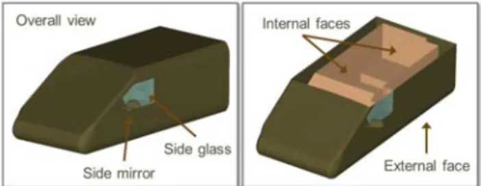
For more information on the SAE body, please refer to [5],[26]. Figure 13 shows the SAE body geometry, the side mirror, side glass and a view of the thickness of the walls.
Figure 13. SAE body: Note the generic shape, side mirror, side glass, outer and inner faces.
4.2 Acoustic Sound power radiated by side glass
To assess the quality of the VA model, an omnisource located inside the SAE body is used to fill the interior volume with acoustic energy. Measurements of pressure inside the SAE body and acoustic intensity on the outer surface of the side glass have been performed. Figure 14 shows that the acoustic power radiated by the side glass is predicted with high accuracy using either BEM or a pure SEA approach. For SEA, prediction has been done up to 10 kHz in a few seconds.
Figure 14. Radiated acoustic power from side glass. Both SEA and BEM are accurate and SEA is computed up to 10
kHz in seconds 4.3 Omnisource outside SAE body
Finally, the omnisource was placed outside the SAE body and predictions and measurements were compared for SPL inside the SAE body using BEM method. Figure 15 shows results for the case where the omnisource is placed at 1 meter and 0°, 45° and 90° from the side glass normal vector. Correlation levels are very high even when the levels vary by as much as 15 dB from one angle to the next for a given frequency. Note that the character of the response is quite different from one location of the source to the next and that the BEM model can properly track the changes in response. The BEM model is especially able to represent the physics for the case where the source is parallel to the side glass. This is quite comforting since this is a configuration very similar to the real life case where the acoustic waves are believed to come from the front of the side glass where the mirror and A-Pillar are located.
Figure 15. Same level of correlation can be observed for the case where source is placed at 1 meter and 0°, 45° and 90° from the side glass normal direction. Note the 15 dB variation from one angle to the other which is captured by
the BEM model.
5. Validation of aero-vibro-acoustic (AVA) models
5.1 Experimental setup
The measurements are described in details in [5]. Figure 16 shows on the left the SAE body in the wind tunnel for the configuration where the vibrations on side glass and SPL inside the SAE body are measured. The middle and right side of the figure shows the surface mounted microphones used to measure the fluctuating surface pressure at the location of the side glass.
Figure 16. Wind-tunnel test: (a) glass module, (b,c) surface microphones over side glass area. 5.2 CFD data
The CFD data used for the prediction of wind noise inside the SAE body is the following:
• StarCCM+ Version 6.06.017
• Half model of an SAE body, a very basic car shape on struts, with/without a side mirror
• Model size: 45 up to 46 million fluid cells • Compressible Detached Eddy Simulation (DES) based on Spalart-Allmaras (S-A)
• Δt CFD = 2E-05s
• First 0.1s of simulated physical time has been cut away: spurious transition phenomena when starting a transient computation based on steady state results
• Flow speed 140 km/h
The pressure time history data was imported into the commercial vibro-acoustics software in [10].
5.3 AVA validation results
The following preliminary results are presented as illustration of the level of correlation that can be achieved for a few configurations. It does not constitute a recommendation of preferred approaches since this is an on-going study as part of the CAA (Computational Aero-Acoustics) German Working Group [5]. The AVA models used are described in details in [27].
Figure 17 shows the average SPL inside the SAE body generated by a 140 km/h wind and the presence of a side mirror predicted using the FE/SEA approach (left) and a BEM approach (right). The modal forces approach was used in combination with CFD compressible data. The FE/SEA predictions are valid starting at around 250 Hz since this corresponds to the first few interior fluid modes represented in SEA. The upper limit is only driven by the number of modes in the FEM glass and the ability of the CFD data to yield accurate representation of the source at higher frequencies. The BEM approach is valid starting at very low frequency because of its deterministic character. It is also valid at quite high frequencies and is only limited by the computation time and memory usage. At this time, BEM computations are presented up to 2250 Hz. Computations to higher frequencies are underway. Both approaches yield highly accurate results for the same CFD input data. Not that the CFD input data quality is paramount to get this level of accuracy inside the vehicle.
Figure 17. Average SPL inside SAE body predicted using FE/SEA Coupled (left) and BEM (right)
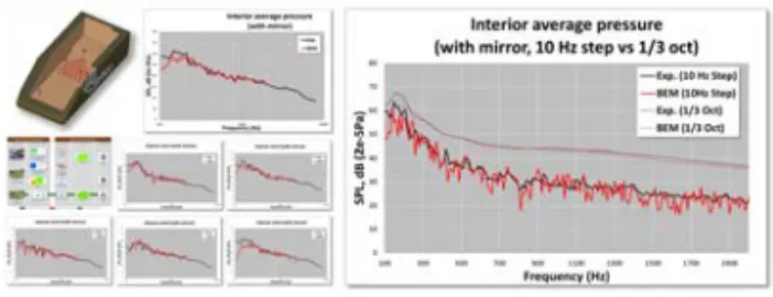
As previously stated, the BEM approach can be used to compare interior microphone SPL predictions with measurements. Figure 18 shows the level of correlation obtained for the configuration with mirror (left). For all microphones, the trend of the curves and levels are well captured. Figure 18 (right) also shows a comparison between measurement and predictions for a 10 Hz frequency step and a 1/3rd octave representation. It can be seen that
the BEM method yields a high level of accuracy when compared with experimental data. Note that in the case of 10 Hz frequency step, the
“peaky” character of the BEM simulation comes from the fact that the CFD simulation has a signal length of less than 0.5 seconds as opposed to the experimental data where the signal was averaged for 30 seconds.
Figure 18. Average SPL inside SAE body generated by 140 km/h wind predicted using a BEM. The wind noise source is represented by modal forces. Note microphone correlation (left) and frequency resolution comparison on
the right.
An important aspect of simulation is the ability of an AVA model to predict various design changes. Figure 19 (left) shows comparisons between the case with and without side mirror. The experimental results for the case without side mirror yield an average interior pressure that is 5 to 10 dB lower than the case with mirror. This trend is also predicted by the AVA model and suggests that the combination of an accurate CFD simulation and an accurate VA model allows the prediction of such a drastic design change.
Figure 19 (right) shows the average SPL inside the SAE body generated by a 140 km/h wind with side mirror predicted using the SEA approach. The contributions from convective and acoustic component were computed from 1D and 2D wavenumber transforms and the total pressure is shown. A single propagating wavefield with an angle corresponding to the rear face of the mirror has been compared with several propagating waves traveling a various angles between 90° and 45° w/r to the side glass normal. Further investigations are underway on this topic and will be reported at a later time.
Figure 19. Left: Comparison of interior SPL with and without mirror using compressible CFD and modal forces.
Right: Comparison of a single and multiple PWF to represent acoustic component of windnoise excitation in combination with a Corcos model for the convective part. The convective component is related to the pressure field generated by eddies travelling at the convection speed. The acoustic component is related to acoustic waves travelling within the flow and being generated on various surfaces before reaching the side glass. The acoustic component is typically very small in amplitude compared to the convective component and as will be shown later in this paper, can be the major contributor at coincidence frequency of the side glass.
Acknowledgements
The authors would like to thank the CAA German Working Group composed of Audi, Daimler, Porsche and VW for authorizing ESI to use their experimental and CFD data for the VA and AVA validation work presented here [5],[26].
References
[1] DeJong R., Bharj T.S., Lee J. J., “Vehicle Wind Noise Analysis Using SEA Model with Measured Source Levels”, SAE Technical Paper 2001-01-1629, 2001.
[2] DeJong R., Bharj T. S., Booz G. G. “Validation of SEA Wind Noise Model for a Design Change”, SAE Technical Paper 2003-01-1552, 2003.
[3] Peng G. C., “SEA Modeling of Vehicle Wind Noise and Load Case Representation”, SAE Technical Paper 2007-01-2304, 2007.
[4] Kralicek, J., Blanchet, D., “Windnoise: Coupling Wind Tunnel Test Data or CFD Simulation to Full Vehicle Vibro-Acoustic Models”, DAGA, Düsseldorf, Germany, 2011.
[5] Hartmann, M., Ocker, J., Lemke, T., Mutzke, A. et al., “Wind Noise caused by the A-pillar and the Side Mirror flow of a Generic Vehicle Model”, 18th AIAA/CEAS Aeroacoustics Conference, Paper 2012-2205, Colorado Springs, USA, 2012.
[6] Arguillat, B., Ricot, D., Bailly, C., Robert, G., “Measured wavenumber: Frequency spectrum associated with acoustic and aerodynamic wall pressure fluctuations”, JASA 128(4), 2010.
[7] Shorter, P., Cotoni, V., Blanchet, D., “Modeling Interior Noise due to Fluctuating Surface Pressures from Exterior flows”, Proc. Society of Automotive Engineers (SAE), ISNVH, 2012.
[8] Shorter, P., Cotoni, V., Blanchet, D., “Modeling interior noise due to fluctuating surface pressures from exterior flows”, ISMA, Leuven, Belgium, 2012.
[9] Bremner, P., Wilby, J., “Aero-Vibro-Acoustics: Problem Statement And Methods For Simulation-Based Design Solution”, Proc. 8th AIAA/CEAS Aeroacoustics Conference, 2002.
[10] VA One 2012, The ESI Group. http://www.esi-group.com.
[11] Cook, R., et al “Measurement of correlation coefficients in reverberant sound fields”, JASA, 27(6), 1955.
[12] Cockburn, J.A., Robertson, J.E., “Vibration Response of Spacecraft Shrouds to In-flight Fluctuating Pressures”, Journal of Sound and Vibration, 1974, 33(4), 399-425.
[13] Larko, J.M., Hughes, W.O., “Initial Assessment of the Ares I–X Launch Vehicle Upper Stage to Vibroacoustic Flight Environments”, NASA Technical Memorandum—2008-215167.
[14] Potschka, N., Callsen, S., “Vibro-acoustic description of a stiffened aircraft structure in flight condition”, ESI Group Vibro-Acoustic User’s Conference (VAUC), Düsseldorf, Germany, 2012.
[15] Orrenius, U., Cotoni, V., Wareing, A., “Analysis of sound transmission through aircraft fuselages excited by turbulent boundary layer or diffuse acoustic pressure fields”, Internoise, Ottawa, Canada, 2009.
[16] Davis, E.B., “By Air by SEA”, Noise-Con, Baltimore, USA, 2004.
[17] Bremner, P. G., Zhu, M., “Recent Progress using SEA and CFD to Predict Interior Wind Noise”. SAE Technical Paper 2003-01-1705, 2003.
[18] Hekmati, A., Ricot, D., Druault, P., “Vibroacoustic behavior of a plate excited by syntesized aeroacoustic pressure fileds”, Proc. 16th AIAA/SEAS Aeroacoustics Conference, AIAA 2010-3950, 2010.
[19] Businger, A. Eberle, M. “Computation of underbody flow aero-acoustics for a production vehicle”, ESI Group Global Forum, Munich, Germany 2010.
[20] Jové, J., Guerville, F., Vallespín, A., “Study Of The Aerodynamic Contribution To The High-Speed Train Cabin Internal Noise By Means Of Hybrid Fe-Sea Modeling”, Internoise, Lisbon, Portugal, 2010,
[21] Shorter, P.J., Langley, R.S., and Cotoni, V., “Aero-acoustics: brief review of the theory adopted in VA One”, VAUC/AVA-SIG: Vibro-Acoustic User’s Conference & Aero-Vibro-Acoustic Special Interest Group, Düsseldorf, Germany, 2012.
[22] Gade, S., Møller, N., Hald, J., Alkestrup, L., “The use of Volume Velocity Source in Transfer Measurements”, Internoise, Prague, Czech Republic, 2004.
[23] Luan, Y., Jacobsen, F., “A method of measuring the Green’s function in an enclosure”. JASA 123(6), June 2008.
[24] Shorter, P.J. and Langley, R.S.: “Vibro-acoustic analysis of complex systems”, Journal of Sound and Vibration, 2004.
[25] Shorter, P.J., and Langley, R.S., “On the reciprocity relationship between direct field radiation and diffuse reverberant loading”. JASA,117, 85-95, 2005.
[26] Hartmann, M., Tokuno, H., Ocker, J., Decker, W. and Blanchet, D., “Windgeräusch eines generischen Fahrzeugmodells: Synchrone Nahfeld-Fernfeld und Nahfeld-Fernfeld-Innenraum Messungen sowie Simulationen”, DAGA, Oldenburg, Germany, 2014.
[27] Blanchet, D., Golota, A., “Wind Noise Source Characterization and How It Can Be Used To Predict Vehicle Interior Noise”. ISNVH, Graz, Austria, 2014.