1)
†To whom correspondence should be addressed.
Han River Flood Control Office, Ministry of Environment E-mail: [email protected]
∙Kwak, Jaewon Han River Flood Control Office, Ministry of Environment / Researcher ([email protected])
Case Study: Groundwater Recharge Hydrograph in Pyeongchang River
Kwak, Jaewon
†Han River Flood Control Office, Ministry of Environment, Seoul, Republic of Korea
평창강 지하수 함양곡선 연구
곽재원
†환경부 한강홍수통제소
(Received : 14 March 2021, Revised : 9 May 2021, Accepted : 16 May 2021)
Abstract
It is important to extract and assess low-flow recession characteristics for water resources management in the upper reaches of a stream. It is difficult to express the groundwater flow recession characteristics for streamflow synthetically. The linear recession model has been widely used by baseflow recession analysis for reason of simplicity and convenience, but recent studies show that nonlinear recession models fit well, and the relationship between the reservoir storage of shallow unconfined aquifers and the groundwater discharge was to be identified as nonlinear in the literature based on the analysis of numerous streamflow recession curves. The objective of the study is to decode these nonlinear characteristics, including evaporation loss, storage, and recharge of groundwater using streamflow. By analyzing the observed time series of streamflow from the study area, which is the Pyeongchang River basin in Korea, the main components of the underlying groundwater balance, namely, discharge, evaporation loss, storage, and recharge, can be identified and quantified. As a result of the study, depletion of groundwater by evapotranspiration losses through the water uptake of tree roots was found to bias the recession curves and the estimated reservoir parameters. The seasonality of both rainfall and potential evaporation, analysis of the recession curves, stratified according to time of the year, allowed the quantification of evapotranspiration loss as a function of a calendar month and stored groundwater storage.
Key words : Groundwater balance, groundwater discharge and recharge, evaporation loss, recession analysis, recession curve 요 약 수자원의 보전과 관리를 위해서는 갈수시의 유량감쇄 특성을 파악하는 것이 중요한 과제 중에 하나이다. 감쇄특성을 하천 유량자료를 이용하여 표현하기 위해서 여러 복잡한 특성을 고려하여야 하므로, 편의성을 위하여 선형 감쇄분석이 주로 적용 되어 왔다. 그러나, 최근의 연구에서 제시된 지하수 유출과 비피압대수층의 저장능력의 비선형성을 고려하면, 비선형 감쇄 모형의 적용성이 더 높다고 할 수 있다. 따라서, 본 연구의 목적은 유출자료를 이용하여 지하수의 증발손실, 저류 및 재함양 과 같은 비선형 특성을 고찰하는 데 있다. 한강의 상류인 평창강 유역의 유출자료를 이용하여 분석을 수행하였으며, 지하수 수지를 구성하는 주요한 요소인 지하수 유출, 증발손실, 저류, 재함양에 대해서 고찰하고 정량화하였다. 연구결과에 따라서, 식생에 의한 지하수 손실이 감쇄곡선을 편향시키는 것으로 나타났다. 또한, 계절적 강우와 잠재증발산 경향을 감쇄분석에 적용하여 월별 증발산 손실과 지하수 함양량을 정량화하여 제시하였다. 핵심용어 : 지하수수지, 지하수 유출 및 함양, 증발손실, 감쇄분석, 감쇄곡선
1. Introduction
It is well known that much of the observed streamflow of many rivers and wetlands in many different hydrological and climatic settings is the outflow from the shallow groundwater reservoirs of the associated basins (Wittenberg and Sivapalan, 1999). Such groundwater reservoirs are important resources both for the maintenance of the natural environment in the wetland as well as for human needs. Therefore, understanding and quantification of the water balance of these shallow groundwater, which take part in the seasonal water cycle, expressed in the form of the time series of storage, discharge and evapotranspiration, recharge, and the relationship of the latter to rainfall inputs, are important (Wittenberg and Sivapalan, 1999). The last remaining component of the groundwater balance is depletion due to evapotranspiration, which may be important depending on climate, soil properties, and especially vegetation (Nichols, 1994). The rate at which a groundwater store discharges in the absence of recharge must be one of the earliest fields of investigation on hydrology, and according to Appleby (1970), has “developed into a closed system of repetitive discovery and rediscovery”. The applications of recession analysis since the early 1900s have been numerous and include such areas as low-flow forecasting, separation of base flow from surface runoff, and the assessment of evapotranspiration loss. An excellent review of the origins and uses of recession analysis is provided by Hall (1986), Tallaksen (1995), and Cuthbert (2014). Also, there are so many studies to contribute the nonlinear characteristics of the groundwater and its assessments (Wittenberg, 2003; Sujono et al., 2004; Rupp and Selker,
2006; Aksoy and Wittenberg, 2011; Thomas et al., 2015; Skaugen and Mengistu, 2016; Jakada et al., 2019). In studies and practical work mostly considered negligible in moderate climate zones, these losses may actually surpass baseflow under arid and semi-arid conditions. However, due to actual change in the pattern of meteorological conditions in Korea peninsula (Choi, 2004), it could not be negligible.
The objective of the study is, therefore, to decode nonlinear groundwater balance characteristics including evaporation loss, storage and recharge using streamflow. The streamflow, rainfall, and evaporation data in the Pyeongchang River basin were obtained, and groundwater balance was analyzed and quantified.
2. Study Area
The case study is performed for the Pyungchang River basin, which is one of the representative basins of the International Hydrological Programme (IHP, 2021). Pyeongchang River is one of the main tributaries and the upper reach of the Han River that flows from north to south. The Pyeongchang River basin has 1,774.32㎢ of basin area (507.2㎢ of upper area), 96.7㎞ of river length, and 39.31 of the average slope. The configuration of the basin is shown in Fig. 1, and there are several hydrological and meteorological stations, groundwater table, and pan evaporation gauges as the facilities for the measurements of hydrologic observations. Daily discharge data of Pyeongchanggun(Sangbangrimgyo), Pyeongchanggun (Sunaegyo) (hereafter referred to as ‘Sangbangrimgyo’ and ‘Sunaegyo’) are used in 1994 to present and daily basin rainfall data during the period are made by the Thiessen method. However, runoff measurement started in 2009 for
Sangbangrimgyo, and 2002 for Sunaegyo, therefore, obtained data was actually used after 2002. Sangbangrimgyo water stage gauge station is located at 128°25´of east longitude and 37°25´of north longitude, and Sunaegyo is 128°24´of east longitude and 37°28´of north longitude. Datum of Sangbangrimgyo and Sunaegyo water level station is 359.2m and 385.4m, respectively. Pan evaporation was obtained from the Yeongwol meteorological station.
3. Baseflow recession analysis and estimation
of storage-discharge relationship
Ever since Mailet (1905), the exponential function
exp has been widely used to describe the baseflow recession, where is the discharge at the time ,
is the initial discharge, and k the recession constant which can be considered to represent average response times in storage. The exponential function implies that the groundwater aquifer behaves like a single linear reservoir with storage linearly proportional to outflow, namely .
It is, however, evident that the parameter k fitted to different discharge ranges of the recession curves in actual rivers dose not remain a constant but increases systematically with the decrease of stream flow (Moore, 1997;), which is a strong indication of nonlinearity. The convenient assumption that the baseflow may be the outflow form, two or more parallel (i.e. independent) linear reservoirs, representing components of different response times is often made (Moore, 1997), and does result in better fits to the observed recession curves. However, this is perhaps only because there are more parameters to be calibrated, giving more degrees of freedoms for curves fitting. In most basins it is unlikely that the dynamic groundwater aquifer can be divided so neatly into such independent storage zones; more likely it consists of a spatially variable (including layered) system of hydraulically communicating pore or fissure systems.
Thus, the use of a single but nonlinear reservoir is considered to be more physically realistic. Nonlinear reservoir algorithm have been proposed and implemented in a large number of basins around world (Wittenberg and Sivapalan, 1999; Chapman, 1997; Brutsaert and Lopez, 1998; Wittenberg, 1994), and are used. To allow for nonlinearity the linear storage-discharge relationship is generalized by adding an exponent b as follows:
∙ (1)
where in and Q in the factor a has the dimension
. If the volumes are expressed in depth, then is
in mm, Q in mm/d and a will be in . The exponent
b is dimensionless. The linear reservoir is a special case of Eq. (1), i.e. when b=1. Combining Eq. (1) with the continuity equation for a nonlinear groundwater reservoir without inflow, i.e. , yields Eq. (1) for the recession curve starting at an initial discharge of , namely :
(2) This corresponds to the expressed in detail in Wittenberg (1999). Given the streamflow recession data the parameter values a and b can be determined by an iterative least squares method (Wittenberg, 1994). By systematically varying the parameter b the value of parameter a is solved at each iteration step, with the condition that the computed outflow volume during the considered time period is equal to that of the observed recession curve. The set of a and b values providing the best fit to the observed curve is considered as representing the properties of the aquifer. Eq. (2) has only one optimal combination of a and b and no restriction was imposed on the value of b. When fitting Eq. (2) to recession data, in almost all cases no significant variation of the parameters a and b was found over different parts of the recession curve, unlike in the linear case, which has been shown to exhibit strong systematic variation (Wittenberg, 1994). The Fig. 2 shows an example of daily runoff and selected recession segment of hydrograph to analyze baseflow characteristics in Sangbangrimgyo. Specifically, the segment that has a continuously decreasing trend from about 1.0mm/day (horizontal line in Fig. 2) during one month was selected.The start of the baseflow recessions had been flow assumed not earlier than two time intervals (days) after the inflection point of the total hydrograph recession. The skewed distribution of the exponent b is peaking between 0.3 and 0.4 with a mean value of b=0.49~0.5 and a standard deviation of 0.25. This empirically estimated mean value
Fig. 2. Daily runoff hydrograph in Sangbangrimgyo in Pyeongchang River.
of 0.5 (i.e. discharge proportional to the square of storage) has also been obtained theoretically for the unconfined aquifers by other authors (Fukushima, 1988). Chapman(1997) found the b values between 0.3 and 0.4 for 10 out of 11 rivers in Eastern Australia, and explained this in low terms of the flow convergence in the groundwater system, Wittenberg(1994) showed for flow recessions of rivers in Germany and China that, on average, a value of 0.4 provided the best fit.
For most practical purposes, such as the regionalization of the relationship given by Eq.(1), it seems reasonable to fix the exponent b at a mean or dominant value, and to allow the coefficient a to vary between basins. A value of b=0.5 is suggested by Wittenberg and Sivapalan (1999) for this purpose, this is especially applicable to hillslope flow-strips (Kubota and Sivapalan, 1995) or to partial basin areas as these are less subject to spatial heterogeneities. It is believed that even if the “true” value of b is not exactly reproduced, the assumption b=0.5 would be more physically realistic and would provide a better match to observed stream flows in a majority of river basins, than the linear reservoir. When fitting the model function with a fixed value of b=0.5 to the German flow recessions an average variation coefficient of CV=7.2% was obtained instead of b (Wittenberg and Sivapalan, 1999).
Wittenberg (1999) shows that the notional value of b=0.5 for the unconfined aquifers is independent of the number of flow strips which make up the basin. He also provides a discussion of the likely causes for the deviation of the field estimates of the exponent b from the theoretical value of b=0.5. Normally (value of a for b=0.5) will be determined from
the observed flow recessions, groundwater losses, e.g. by evapotranspiration, however, can have a biasing effect, lowering the computed so that this factor will no longer represent
the true storage-discharge relationship of the aquifer. The analysis is performed in two ways. One is for two exponents (a and b) and the other is for one exponent (a with a fixed b=0.5). The estimates of are represented in Table 1 with
its simulation efficiency using RMSE and R2 (Hyndman and Khandakar, 2006). From the calibrated curves in Fig. 3, the fitted curve by two exponents is better than by one exponent but there are no large differences between the fitted curves. Therefore, one exponent is considered for practical purpose and simplicity of nonlinear reservoir modeling. The mean seasonal variations of pan evaporation are shown in Fig. 4. The data series show seasonal monsoon climate which is high temperature and evaporation in summer and low temperature and evaporation in winter. Therefore, the variation of data series shows sinusoidal pattern.
Table 1. Selected segments and estimated exponent for nonlinear
reservoir modeling
Station N Segments RMSE R2
Sang bang rim gyo 1 May-2014 49.1 0.029 0.94 2 Jul-2014 31.4 0.058 0.95 3 Jul-2015 50.4 0.004 0.99 4 Sep-2015 34.0 0.035 0.97 5 Aug-2016 28.1 0.029 0.89 6 Sep-2016 39.4 0.049 0.85 7 Apr-2017 50.3 0.077 0.80 8 May-2018 37.1 0.052 0.84 9 Nov-2020 20.6 0.034 0.92 10 Oct-2020 50.0 0.075 0.95 Sunae gyo 1 May-2014 71.1 0.013 0.95 2 Jul-2015 32.7 0.113 0.84 3 Jun-2017 31.6 0.069 0.89 4 Sep-2017 47.7 0.044 0.90 5 May-2020 40.0 0.076 0.87
Fig. 3. Comparison of observed data and nonlinear reservoir models.
Fig. 4. Seasonal variation of pan evaporation (Pyeongchang River basin).
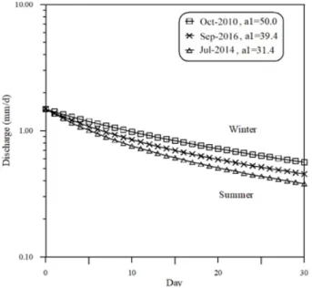
Seasonal recession curve may vary with evapotranspiration as shown in Fig. 5. Fig. 5 shows the recession curves extracted from the observed daily flow for the different seasons and significant seasonal variations of with ordinary water level
(2mm/day). The curves describe the faster recession and a smaller value of in summer and a slower recession and
a larger in winter.
The Fig. 6 shows the seasonal variation of and it shows a tentative sinusoidal curve as fitted. Hence, the observed seasonal variation of the coefficient suggests that the
baseflow is not the only outgoing water flux from the groundwater reservoir. A seasonally varying rate of
Fig. 5. Seasonal variations of recession curve (Pyeongchang River).
Fig. 6. Seasonal variation of parameter .
evapotranspiration loss from the groundwater aquifer appears as the most probable and plausible cause for the changing steepness of the streamflow recession. Baseflow recession studies in the Pyeongchang River, suggest a strong seasonal variation of the storage-discharge relationship of the shallow aquifers, which can be attributed to biasing by seasonally varied evapotranspiration losses. When the Fig. 5 and Fig. 6 are compared, it is evident that pan evaporation and estimated variation of have the strong negative correlation. Table 2
represents the values of in each month obtained from the
Fig. 6.
4. Estimation of evapotranspiration
The depletion of groundwater storage by evapotranspiration, or through fluxes other than baseflow, results in a biased streamflow recession curve which decreases at a faster rate than if would be expected with the “true” reservoir coefficient . This is demonstrated in Fig. 7 by two hypothetical recession curves for Pyeongchang River, starting from an arbitrary value . The upper recession would occur
under winter conditions (July) which is subject to minimum losses, and here assumed to be zero, and under summer conditions (January) with maximum losses.
For every time interval Δt evapotranspiration loss can be determined as the difference between the theoretical (i.e. potential) storage ∙ which would have
occurred at the end of the time interval with minimum evapotranspiration loss, and corresponding to theoretical baseflow discharge , and the actual storage ∙
(subject to increased losses). Note that , being the “true”
unbiased reservoir coefficient, determines the true storage corresponding to outflow in any season. That is,
∙ or ∙ is hydraulic-volumetric
hence physical relationships for the reservoir. However, parameter is unbiased, and is smaller only because
the additional evapotranspiration loss makes the baseflow recession curve steeper. Hence, if one wants to estimate this steeper recession curve, then must
be used, as in Eq.(3). In terms of a groundwater balance equation a preceding storage value would become, after a time interval Δt = 1 day, at time i (i.e. on the i th day):
Table 2. The average values of for each month of the year
Month 1 2 3 4 5 6 7 8 9 10 11 12
(3)
with only baseflow and
(4)with baseflow and evapotranspiration . For simplicity we define in terms of daily depth. Note that both the terms on the right side relate to real (physical) storage, not biased ones. is discharge (during a recession) when
is minimum, and is the discharge during recession which is influenced by evapotanspiration. Starting from the preceding baseflow , the value is obtained according to Eq.
(2) using the constant (minimum “no” losses, December),
while is computed with (increased evaporation losses)
thus becomes:
(5) Replacing yield Eq. (6) which shows
clearly that evapotranspiration losses from the groundwater depend on season via the factor and groundwater volume
which is related to groundwater depth:
(6)
Fig. 7. Estimation of groundwater evapotranspiration (Pyeongchang River).
The relationships between evapotranspiration loss and storage depth of the groundwater can be computed by Eq. (6) using the average values of for each month of the
year as given by the sinusoidal curve. Two hypothetical recession curves starting from average of selected
segments for Pyeongchang River are shown in Fig. 7. It is also considered that upper recession curve would occur under winter conditions (December), which is subject to minimum losses (assumed to be zero), and the lower recession would occur under summer conditions (June) with maximum losses. Evapotranspiration is assumed by the difference of recession curve.
5. Inverse modeling through baseflow
separation
There are many techniques for baseflow separation, though while most procedures are based on physical reasoning, the quantitative elements of the separation techniques are essentially arbitrary. Useful reviews of base flow separation techniques are presented by Hall(1971). The nonlinear reservoir algorithm was also applied for the separation of baseflow from time series of total daily streamflow from time series of total daily streamflow. The procedure and application has been amply described by Wittenberg (1999). The computation starts at the last value of the time series and proceeds backwards along the time axis. A flow recession at the time ∆ is determined from the flow at the time using Eq. (7), which has been derived by inverting Eq.(2). The time step ∆ is normally one day.
∆
∆
(7) Recession periods of the flow hydrographs are disrupted by the recharge periods. Baseflow will then rise and we need to develop a scheme to connect the preceding lower baseflow values to the higher baseflow values which follow after the new storm event recharges the groundwater reservoir. Recharge volume and the duration of recharge can be determined from the difference between the aforementioned recessions. As recharge is usually coincident with the rising and peaking of total flow, the following approach was adopted (Wittenberg, 1999). When the reverse computed baseflow recession curve intersects the rising limb of the total hydrograph, a transition point which is at the next time step forward from the total flow is adopted as the peak of baseflow. Values of the rising limb of the baseflow hydrograph are then found as the computed recession curve
for one time step forward for each given total flow value. This procedure is similar to the digital filter described by Chapman (1997) for baseflow separation for the linear reservoir.
According to Wittenberg (1999), the peak of baseflow is occurred at the peak point of runoff hydrograph. However, the method by Wittenberg (1999) to separate baseflow from runoff hydrograph is not consistent with the hydrograph from the Pyeongchang River basin. Therefore, we propose a method here to separate the baseflow from the runoff hydrograph by considering the relationship between streamflow and groundwater stage. Eq.(8) proposed in this study can be used for the aim of the baseflow separation for obtaining the points from the starting of rising limb to the peak of the baseflow.
×
(8) is the start day of rising limb of runoff hydrograph
which is considered as the start day of groundwater flow.
is the baseflow for the peak day corresponding to the groundwater stage. is the surface flow.
Each hydrograph for eleven single storm events is selected to separate the components of hydrograph in Sangbangrimgyo water stage as shown in Table 3 and the groundwater recharge is estimated. The Fig. 8 shows an example of hydrograph separation. It is assumed that groundwater stage has relationship with baseflow quantity as demonstrated. We consider the surface runoff and
Fig. 8. Baseflow separation considering groundwater stage.
Table 3. Total rainfall, effective rainfall, runoff rate and Φ-Index
N Month Total (mm) Effective (mm) Runoff rate Ф-Index (mm) 1 Nov-2009 108.0 30.8 0.286 26.1 2 Sep-2010 99.4 33.6 0.338 20.8 3 Jul-2014 273.3 39.4 0.144 97.2 4 Oct-2014 48.5 12.3 0.253 21.5 5 Aug-2015 109.0 75.0 0.688 22.7 6 Aug-2015 144.2 67.1 0.466 55.8 7 Jul-2017 103.2 39.2 0.380 45.5 8 Aug-2017 182.2 60.9 0.334 34.0 9 May-2018 26.8 18.6 0.693 3.9 10 Oct-2018 100.4 13.5 0.134 41.9 11 Oct-2018 43.9 5.6 0.129 20.4 Average 0.350 35.4
groundwater stage to separate the baseflow from the surface runoff. Say, the baseflow is separated from the surface runoff by considering the same pattern as groundwater stage. The increment of the baseflow, ∆, may be proportional to the increment of surface runoff, , as shown
in Fig. 8. It is known that the fluctuation of runoff rate is large from the Table 3 and it is due to the small peak time of Pyeongchang River basin. Daily discharge measurement cannot express storm event characteristic by rainfall exactly. That is, as difference of discharge measurement time of water stage and dropped rainfall time is larger, as variation of runoff rate is smaller in the contrary. The effective rainfall is needed to estimate the groundwater recharge response function and this study uses Φ-index method. As shown in Table 4, the fluctuations of Φ -index are large.
6. Groundwater recharge response to rainfall
and its application
Based on the obtained baseflow by Eq.(8), the effective groundwater recharge is computed for every time step as follows:
(9)
where S is the actual storage computed by Eq.(1) using the unbiased storage factor . For practical computation
the baseflow volume during this time interval is determined by the trapezoidal formula, thus
≈ ∆
. Evaportanspiration losses () from the groundwater are
computed using Eq. (6) with daily values of . As every
rainfall impulse appears to produce a similar response, differing of course in magnitude, it appears reasonable to apply a linear unit response function of the unit hydrograph type. Linear response functions to estimate recharge have been derived. The assumption of linearity for the transfer of infiltrated rainwater, through the unsaturated vadose zone to the groundwater Table, appears reasonable because the conductivity of that zone can be assumed not to vary significantly with time when water percolates through it (Besbes and de Marsily, 1984). For the same reason, time invariance can also be expected. Under these two conditions, recharge GWS from infiltrating rainfall can be estimated by the application of the convolution integral:
∙ (10)
where is the unit response function, which is defined as the theoretical recharge hydrograph which would occur for 1mm of effective rainfall percolation through the groundwater surface. For practical computations, with digital data of a time interval ∆, the convolution integral becomes:
∙ ∆ (11) Where and are in mm. In this study effective rainfall has been assumed proportional to measured rainfall throughout each recharge event. As the time interval for computations is ∆ day, the response function in Eq.(11) represents a travel time distribution in . For
every sequence of values of effective rainfall there is
a corresponding sequence of value of recharge , which could be computed by convolution, i.e. multiplication of the response function with every value and time shifted superposition of the estimated recharge hydrographs. The length or number of value of the response function
is thus . Eq. (11) thus represents a system
of n linear equations with unknowns , which
can be resolved by the least squares method (Snyder, 1955). Generally groundwater recharge is affected by infiltrating rainfall of Eq. (10), but the baseflow is separated from surface runoff by considering the pattern of groundwater stage. Also, groundwater recharge may be more related to effective rainfall than infiltrating rainfall because groundwater recharge is proportional to the increase of baseflow which is related to the surface runoff and the surface runoff is related to the effective rainfall. Therefore, the groundwater recharge equations of Eq. (10) and Eq.
(11) representing infiltrating rainfall should be changed as the function of effective rainfall. Merely, evapotranspiration losses () that are represented in Eq. (6) and Eq. (9~11) are considered in intermittent rainfall periods. In fact, monsoon periods are generally shown zero or similar value of evaporation. Therefore, these equations for groundwater recharge could not be applied for monsoon periods.
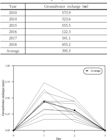
The Fig. 9 shows the groundwater recharge response function for 1mm-effective rainfall of 1 day and the function can be computed from rainfall and recharge events for each month of the year in Pyeongchang River basin. Then, hydrographs of groundwater recharge are recomputed by convolution of the response function with measured rainfall in the following section. The shape of the determined functions is very similar. The travel time distribution thus appears rather time invariant not only within the events but also over all seasons. Peak recharge is reached at the first day after the rainfall event and recharge ends after 2~3 days. The similarity of the response functions allows the derivation of a typical mean unit response function by averaging. Concerning the recharge functions obtained in this study, the shape will be influenced by baseflow modeling during the recharge phase. The length is restricted by the basic assumption of baseflow separation that there is no
Table 4. Groundwater recharge for year
Year Groundwater recharge (㎜)
2010 573.9 2014 323.6 2015 555.5 2016 122.3 2017 341.1 2018 455.2 Average 395.3
Fig. 9. Response function of groundwater recharge for
Fig. 10. Groundwater recharge hydrograph computed from effective rainfall for Pyeongchang River basin in July, 2010.
further recharge when typical recession starts. The comparatively long recession of the recharge functions derived in other studies, however, may be partially due to the adoption of the cascade of linear reservoirs as a model function for which the long tail is to be expected.
Fig. 10 shows groundwater recharge in summer by the response function of effective rainfall. The Φ-index to calculate effective rainfall uses the average value in Table 3. This method can estimate groundwater recharge by knowing effective rainfall which is calculated by a Φ-index. Monthly or seasonal groundwater recharge quantity will be taken by in this method corresponding to this duration. Yearly groundwater recharge is shown in Table 4 by this method.
7. Conclusion
The groundwater balance of a basin and the processes of recharge, storage, evapotranspiration loss and discharge can be described by simple but physically based conceptual model components. The properties of these components can be identified and obtained from streamflow data. Observed streamflow data especially for flow recessions are considered as a very authentic database for a basin, carrying a wealth of information about the foregoing hydrological processes. Decoding some of this information is the main purpose of this work. The nonlinearity of the storage-discharge relationships has been found in the literature. Depletion of the groundwater aquifer by evapotranspiration losses, however, biases the observed flow
recession curves depending on the storage, vegetation and potential evapotranspiration. Although these losses are known and acknowledged in the past literature (Tallaksen, 1995) they have been rarely considered in the recession analysis; as shown in this study, baseflow recession analysis also permits their quantification. Pan evaporation during winter in Pyeongchang River basin is almost 1.5~2.0mm daily. The Eq. (2-15) must be changed to consider winter evapotranspiration. The complexities of basin processes are such that the applications described in this study are not expected to accurately reflect baseflow or recession performance. The term “baseflow” itself is more of a conceptual convenience than a precise description of the nature of the source. In this study, baseflow quantity is assumed that concerned with groundwater stage and baseflow separation is performed roughly by the shape of groundwater stage. However, a precise quantitative analysis is required about relationship between surface flow and groundwater stage in many other basins. If relationship between surface flow and groundwater stage according to basin geology characteristics can be identified clearly, groundwater recharge will be estimated easily by the method proposed in this study. By including evapotranspiration flux in baseflow separation techniques, hydrographs of recharge to the aquifer were computed by inverse nonlinear flow routing. Linear time-invariant unit response functions were identified between the measured rainfall and the recharge hydrographs estimated by the baseflow separation.
References
Appleby, V. C. (1970). “Recession and baseflow problem”, Water Resources Research, 6(5), pp. 1398-1403. Aksoy, H., and Wittenberg, H. (2011). Nonlinear baseflow
recession analysis in watersheds with intermittent streamflow. Hydrological Sciences Journal, 56(2), pp. 226-237. https://doi.org/10.1080/02626667.2011.553614 Besbes, M., de Marsily, G. (1984). From infiltration to
recharge: use of a parametric transfer function. Journal of hydrology. 74, pp. 271-293. https://doi.org/10. 1016/0022-1694(84)90019-2
Brustsaert, W.H., Lopez, J.P. (1998). Basin-scale geohydrologic drought flow features of riparian aquifers in the southern Great Plains. Water Resources Research, 34(2), pp. 233-240. https://doi.org/10.1029/97WR03 068
Chapman, T. (1997). A comparison of algorithms for streamflow rcession and baseflow separation. In: McDonald, A.D., McAleer, M. (Eds.), Proceedings of international Congress on Modelling and Simulation
MODSIM 97. Hobart, Tasmamia, Australia, pp. 294-299.
Choi, YE. (2004). Trends on temperature and precipitation extreme events in Korea. Journal of the Korean Geographical Society, 39(5), pp. 711-721
Cuthbert, M. O. (2014). Straight thinking about groundwater recession. Water Resources Research, 50(3), pp. 2407-2424. https://doi.org/10.1002/2013 WR014060
Fukushima, Y. (1988). A model of river flow forecasting for a small forested mountain catchment. Hydrological processes, 2, pp. 167-185. https://doi.org/10.1002/ hyp.3360020207
Hall, A.J. (1971). Baseflow recessions and baseflow hydrograph separation problem, In Hydrology Symposium of Institution of Engineers, Australia, Canberra, pp. 150-170.
Hyndman, R.J. and Khandakar, Y., (2006). Automatic time series for forecasting: the forecast package for R (No. 6/07). Monash University, Melbourne: Department of Econometrics and Business Statistics. Melbourne, Australia.
International Hydrological Programme (IHP) Korean National Committee (2021). http://www.ihpkorea.or. kr/eng/info_05.html
Jakada, H., Chen, Z., Luo, M., Zhou, H., Wang, Z., and Habib, M. (2019). Watershed characterization and hydrograph recession analysis: a comparative look at a karst vs. non-karst watershed and implications for groundwater resources in Gaolan River Basin, Southern China. Water, 11(4), pp. 743. https://doi.org/10.3390/ w11040743
Kubota, J., and Sivapalan, M. (1995). Towards a catchment‐ scale model of subsurface runoff generation based on synthesis of small‐scale process‐based modelling and field studies. Hydrological Processes, 9(5‐6), 541-554. Maillet, E. (1905). Essai d’hydraulique souterraine et
fluviale: Librairie scientifique. Hermann, Parid. Moore, R.D. (1997). Storage-outflow modeling of
streamflow recessions with application to a shallow-soil forested catchment. Journal of hydrology, 198, pp.
269-270
Nichols, W. (1994). Groundwater discharge by phreatophyte shruvs in the Great Basin asa related to depth to groundwater. Water Resources Research, 30, pp. 3265-3274.
Skaugen, T., and Mengistu, Z. (2016). Estimating catchment-scale groundwater dynamics from recession analysis–enhanced constraining of hydrological models. Hydrology and Earth System Sciences, 20(12), pp. 4963-4981. https://doi.org/10.5194/hess-20- 4963-2016
Sujono, J., Shikasho, S., and Hiramatsu, K. (2004). A comparison of techniques for hydrograph recession analysis. Hydrological processes, 18(3), pp. 403-413. https://doi.org/10.1002/hyp.1247
Synder, W.M. (1955). Hydrograph analysis by the method of least squares. J. of Hydraul. Div., Amer. Soc. Civ. Engrs., 81, pp. 793
Tallaksen, L.M. (1995). A review of baseflow recession analysis. Journal of hydrology, 165(1-4), pp. 349-370. Thomas, B. F., Vogel, R. M., and Famiglietti, J. S. (2015).
Objective hydrograph baseflow recession analysis. Journal of hydrology, 525, pp. 102-112. https://doi. org/10.1016/j.jhydrol.2015.03.028
Rupp, D. E., and Selker, J. S. (2006). Information, artifacts, and noise in dQ/dt− Q recession analysis. Advances in water resources, 29(2), pp. 154-160. https://doi.org/ 10.1016/j.advwatres.2005.03.019
Wittenberg, H. (1994). Nonlinear analysis of flow recession curves. IAHS Publications-Series of Proceedings and Reports-Intern Assoc Hydrological Sciences, 221, 61-68.
Wittenberg, H., and Sivapalan, M. (1999). Watershed groundwater balance estimation using streamflow recession analysis and baseflow separation. Journal of hydrology, 219(1-2), pp. 20-33. https://doi.org/10. 1016/S0022-1694(99)00040-2
Wittenberg, H. (2003). Effects of season and man‐made changes on baseflow and flow recession: case studies. Hydrological processes, 17(11), pp. 2113-2123. https://doi.org/10.1002/hyp.1324