A multi-dimensional crime spatial pattern analysis and prediction model based on classification

272

|

1

|

INTRODUCTION

Decades of study have firmly established that crime shows geographical (ie, spatial) patterns [1]. Analysis of spatial pat-terns is a standard research approach in criminology, just as it is in ecology, epidemiology, and other fields. Spatial pat-terns may have different dimensionalities, as they can involve points, lines, or areas; they may also vary with resolution. Crime-pattern analysis may be conducted at the level of cen-sus tracts, zip-code units, street segments, counties, states, or countries. In this work, after considering a number of possi-ble resolutions, we find and utilize one that seems optimal for crime prediction.

Spatial pattern analysis can be density-based (area-based) or distance-based. However, Euclidean distance is not al-ways useful in identifying urban crime patterns: Places that

are close together on a map (in terms of Euclidean distance) may in fact be very isolated from each other if they are not joined by streets, are on opposite sides of a river with few bridges, or are in neighborhoods separated by some invisi-ble economic or social barrier that keeps residents apart. On the other hand, density- or area-based spatial pattern analysis seems to fit naturally with the intuitive concept that cities are built up of neighborhoods. Density-based analysis can be further categorized as global or local. The first considers the ratio of observed crime events to the area of the region under study; the latter measures crime incidence for different units within that region.

The spatial pattern is only one aspect of the distribution of crime; there are also temporal patterns. Many researchers have studied variation in crime rates between day and night, weekday and weekend, or among different seasons of the

O R I G I N A L A R T I C L E

A multi-dimensional crime spatial pattern analysis and

prediction model based on classification

Gaurav Hajela

_|

Meenu Chawla

_|

Akhtar Rasool

Engineering, Maulana Azad National Institute of Technology, Bhopal, India

Correspondence

Gaurav Hajela, Department of Computer Science and Engineering, Maulana Azad National Institute of Technology, Bhopal, India.

Email: [email protected]

Abstract

This article presents a multi-dimensional spatial pattern analysis of crime events in San Francisco. Our analysis includes the impact of spatial resolution on hotspot identification, temporal effects in crime spatial patterns, and relationships between various crime categories. In this work, crime prediction is viewed as a classification problem. When predictions for a particular category are made, a binary classifica-tion-based model is framed, and when all categories are considered for analysis, a multiclass model is formulated. The proposed crime-prediction model (HotBlock) utilizes spatiotemporal analysis for predicting crime in a fixed spatial region over a period of time. It is robust under variation of model parameters. HotBlock's results are compared with baseline real-world crime datasets. It is found that the proposed model outperforms the standard DeepCrime model in most cases.

K E Y W O R D S

classification, ensemble learning, hotspot analysis, spatiotemporal analysis

This is an Open Access article distributed under the term of Korea Open Government License (KOGL) Type 4: Source Indication + Commercial Use Prohibition + Change Prohibition (https://www.kogl.or.kr/info/license.do#05-tab).

year [2,3]. Crime spatial patterns are sometimes governed by their temporal aspect. For example, in countries with cold winters, pickpockets will go to the beach only during the summer when there are large crowds and not in winter when the beach is empty. Spatiotemporal patterns thus depend on many factors: weather, census parameters, the environment, the points of interest in an area, and more.

The goal of spatiotemporal analysis of crime patterns [4] is to find hotspots [5], that is, areas on the map where the concentration of crime is higher than elsewhere. Hotspots can have various dimensionalities. They can be zero-dimensional if the crime occurs at very specific places. For example, a map showing the location of bank robberies will typically show the locations of various banks as dots. A discrete loca-tion (example: bank) at which crimes are frequent is called a hotplace, and in analysis is typically shown on a map with a dot, the size of which is proportional to the number of crime events at that place. Thus, a frequently robbed bank would be shown by a large dot, while a never-robbed bank would be shown by a tiny one. In one-dimensional hotspot analysis, a street (linear structure) is identified as the hotspot. In two-di-mensional hotspot analysis, by contrast, hotspots may have any shape: circular, elliptical, rectangular, polygonal, etc. They are often chosen to coincide with zip-code units, census tracts, or political districts.

We have undertaken spatiotemporal analysis of crime pat-terns in New York and San Francisco; however, only spatial analysis for San Francisco is discussed in the present paper. The spatial analysis is done at four levels: census tract, zip-code unit, district, and grid block (HotBlock Approach). The hotspot units at each level of analysis are identified. We also study daily, weekly, and seasonal variations in the crime rates of these hotspot units. A crime-prediction model based on spatiotemporal analysis is proposed, and its performance is evaluated for datasets from New York and San Francisco.

2

|

LITERATURE REVIEW

Andresen [6] performed a spatial analysis of crime events that occurred in Vancouver, Canada. Crime rates in different spa-tial regions were calculated and interpreted from a standpoint integrating two of the most popular theoretical frameworks in criminology: social disorganization theory and routine-ac-tivity theory. Instead of utilizing the residential population of the spatial region to calculate the crime rate, the author sug-gested employing the ambient population, a better measure of the expected number of people in any region at any given time. The crime rates for three categories (auto theft, break-ing and enterbreak-ing, and violent crime) were calculated usbreak-ing both the residential and the ambient populations; it was found that the ambient population represented the population at risk better than the residential.

Later, Andresen [7] investigated the importance of imme-diate spatial neighbors in local crime-pattern analysis. Some of the standard methods used for spatial pattern testing, such as Moran's I, are global in nature, that is, they give a single statistic for the whole study area, even though the study area is a collection of many small regions. This can be problematic when a statistically insignificant area adjoins an area of high importance. For this reason, Andresen used Local Indicators of Spatial Association (LISA) [8] to classify regions as local clusters.

Cowen and others [9] performed a spatiotemporal analysis of crime events in Miami-Dade County neighborhoods. The model predicted crime patterns in space and time based on land use and walkability. Ordinary least squares regression and spatial analysis incorporating social disorganization theory and routine-activity theory were used to investigate the relationship of land use and violent crime rates. A walkability index was calculated based on four factors: distance from public transpor-tation, distance from bike lanes, street intersection density, and access to amenities. It was found that higher walkability was correlated with a greater number of aggravated assaults, while increase in land-use diversity was correlated with increases in both aggravated assault and larceny.

Vildosola and others [10] applied risk terrain modeling to residential and vehicle burglary rates in Coral Gables, Florida. The focus of their work was to verify that risky places identi-fied by the sociological model were indeed high crime areas. This information could be used to predict future hotspots for more efficient deployment of resources. To identify risky places within the study area, various risk factors (the number of alcohol vendors, car dealers, gas stations, bars, schools, grocery stores, and restaurants) were considered. Regression was used to provide a weight corresponding to each risk fac-tor. It was found that risky places identified by the study had high crime rates according to police records.

Zheng and others [11] have proposed a novel framework for crime prediction based on neural networks. Their model, named DeepCrime, considers all the dynamics of crime and has been found to be considerably more efficient than state-of-the-art baselines. The DeepCrime model frames a crime matrix representing all (in the study, four) categories of crime sequences across specified time slots in a region. DeepCrime was tested on a dataset from New York. The sensitivity of the model was tested by varying each parameter while keeping the others fixed. It was found that DeepCrime was robust and that there was no major performance degradation with small changes in parameters.

3

|

PROPOSED METHODOLOGY

This research addresses the following questions: (a) Is there any correlation between crimes in different crime

categories or are crime events completely independent? (Section  3.2) (b) Is there any relation between the char-acteristics of the community in an area and the prominent category of crime in that area? (Section 3.2) (c) Does the resolution level of the spatial analysis have any impact on hotspot results? (Section 3.3) (d) Is there a temporal influ-ence on crime spatial patterns? (Section 3.4) (e) Can spa-tiotemporal analysis be used to create a crime-prediction model? (Section 3.5) (f) If so, is the prediction model sen-sitive to the spatiotemporal parameters used for analysis? (Section 4.3).

3.1

|

Dataset description

As discussed in Section  1, there are many indicators that could be considered in relation to the crime rate, among them weather indicators, social media indicators [12,13,14], census-based indicators, and crime history indicators. In this work, the last two are considered for analysis. The proposed models and other baselines are evaluated on the following datasets:

1. San Francisco Crime Dataset: This dataset contains crime events collected from January 2014 to December 2014 with 37 different categories of crime. Of these, 13 contain a sufficient number of instances for evaluation of proposed models and analysis.

2. New York City (NYC) Crime Dataset: This dataset contains crime events collected from January 2014 to December 2014 with 68 different categories of crime. Of these, only four are selected. The same set of four crime categories is taken in the baseline (DeepCrime [11]) with which we have compared our proposed model.

3. San Francisco Census Dataset: The San Francisco Crime Dataset contains police department districts, while census data are organized by zip code. These data must be prop-erly aggregated according to districts to be used for analy-sis. From the census data, we extract information about how many people in the districts of San Francisco have a high annual income (more than $50 000), are below the poverty line, have a low (less than 12th grade) educational level (males only), or live in high-priced housing (costing more than $500 000).

3.2

|

Crime rates for each category and

correlation analysis for San Francisco

San Francisco is divided into districts for policing. The popu-lation of each district can be found from the census dataset. The census statistics are reported according to zip codes; by taking zip codes falling within a district as a unit, a dataset

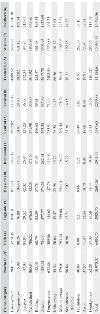
can be prepared from census statistics which contains dis-trict-wise population. This dataset along with the crime data-set is utilized to calculate crime rates for each category under study, as shown in Table 1.

It can be inferred from the Table 1 that the Mission and Southern districts have the highest crime rates, whereas Taraval, Bayview, Ingleside, and Richmond are on the low side. Theft is least common in the Bayview district, which has the smallest percentage of the population having a high income. Tenderloin has a large percentage of the population having low education and below the poverty line; it also has major drug, assault, robbery, and trespass problems. These results verify social disorganization theory which relates the characteristics of the community living in an area with the category of crime and the crime rate [15]. It is observed that the percentage of the population below the poverty line and the percentage of the male population having low education tend to be similar in every district (ie, a district that has a low percentage of the male population with little education typically has a low percentage of the population below the poverty line, as shown in Figure 1). High housing price (more than $500 000) and high annual income (more than $50 000) are also distributed similarly across the districts, as shown in Figure 2. (The thresholds for high income and housing price are simply the average values taken from San Francisco cen-sus data.). However, Northern (#2) and Ingleside (#9) dis-tricts are anomalous on both charts.

Only 13 out of 37 crime categories have a sufficient num-ber of instances for correlation analysis. The Pearson correla-tion coefficient is calculated between all pairs of these 13 categories; total crime instances are also treated as a separate category. It is clear from Table 2 that every crime category is positively correlated with every other across the districts. The correlation coefficient is high especially for certain pairs: Robbery and Weapons Law, Robbery and Trespass, Assault and Weapons Law, Drunkenness and Sex Offences (Forcible). On the other hand, the correlations between Drugs and Vehicle Theft, Prostitution and Theft, Prostitution and Drugs, and Drunkenness and Theft, although positive, were very low.

3.3

|

Crime spatial pattern analysis for

San Francisco

As discussed in Section  1, spatial pattern analysis can be done at different resolutions. This study aims to iden-tify the impact of spatial resolution on hotspot detection. Spatial pattern analysis is done at three resolutions, namely at census tract, zip-code, and district level. (In Section 3.5, a grid-based approach (the HotBlock Approach), which operates at yet another spatial resolution, will be intro-duced.) The finest resolution of spatial analysis is census

tract level, as shown in Figure 3. In this work, we perform polygon density analysis, a neighborhood-based statistical method that provides a density of crime events within each polygon (raster cell). A raster cell can be a census tract, a zip-code area, a district, or even the complete study area. The ranges shown on the left of all spatial pattern maps represent crime density. In all the analyses performed in this work, only properly geocoded crimes were included in the study and crime events are geocoded with more than acceptable hit rate [16].

In the previous section, crime rates per district were cal-culated and discussed. While crime rates take the population of the district into account, polygon density maps consider the area. It can be inferred from the spatial analysis at the

FIGURE 1 Correspondence between percentages of the

population having low education (males only) and living below the poverty line across districts of San Francisco

0 5 10 15 20 25 1 2 3 4 5 6 7 8 9 10 % by population Districts Low education Below poverty line

FIGURE 2 Correspondence between percentages of population

having an income over 50 000 and living in houses costing over 500 000 across districts of San Francisco

0 5 10 15 20 25 30 35 40 45 1 2 3 4 5 6 7 8 9 10 % by populatio n Districts High income High house price

TABLE 1

Crime rates (per 100 000 inhabitants) for crime categories across districts of San Francisco

Crime category Northern (2) a Park (4) Ingleside (9) Bayview (10) Richmond (1) Central (3) Taraval (8) Tenderloin (5) Mission (7) Southern (6) Larceny/theft 7091.75 3279.06 979.18 877.20 1832.18 3912.82 1132.42 4389.52 5488.85 10 350.70 Weapons law 115.99 80.26 76.00 104.40 15.72 54.81 29.00 282.02 431.12 199.74 Trespass 147.03 84.84 29.52 42.02 26.94 127.23 36.78 212.34 384.83 213.67 Vehicle theft 865.84 786.52 676.64 432.03 371.60 371.90 350.83 301.92 1955.96 645.66 Robbery 145.40 68.79 85.59 57.78 37.05 106.68 39.61 255.47 361.68 193.54 Assault 1354.31 754.41 577.77 574.51 282.91 763.38 337.39 2617.78 3503.95 1927.69 Drug/narcotic 633.86 509.06 144.63 187.78 119.00 233.91 71.44 2405.44 1550.88 904.23 Kidnapping 55.54 20.64 32.47 22.98 15.72 28.38 14.15 66.36 101.27 52.64 Missing person 379.01 793.40 259.00 254.10 194.22 209.44 178.24 391.51 1385.96 743.21

Sex offenses (forcible)

50.64 38.98 17.71 17.07 15.72 37.19 14.15 76.31 199.65 74.32 Prostitution 40.84 0.00 2.21 0.66 2.25 69.49 2.83 19.91 263.30 37.16 Arson 37.57 11.47 12.54 19.70 8.98 18.60 8.49 19.91 72.34 38.71 Drunkenness 52.28 57.33 15.50 14.44 19.09 53.83 15.56 116.12 283.56 114.58 Total 10 970.07 6484.75 2908.75 2604.68 2941.37 5987.65 2230.88 11 154.61 15 983.33 15 495.86

aDistrict numbers mentioned in brackets are used in

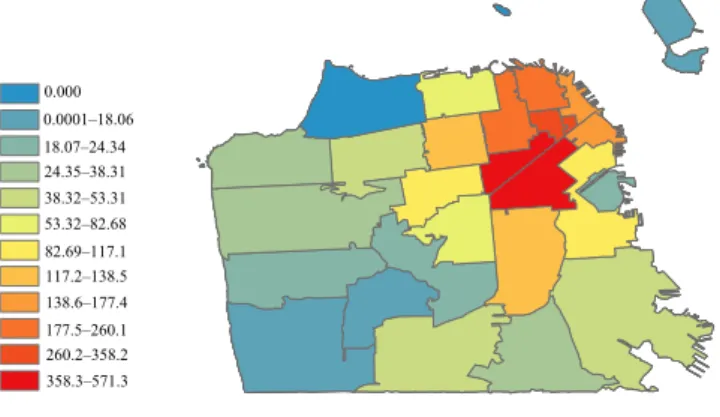
census tract level, zip-code level (Figure 4), and district level (Figure 5) that areas identified as hotspots in analysis at one resolution might not be so identified at another, for example, when a small area with a high crime rate is surrounded by a large area with a very low one. This is why the selection of the level of analysis (resolution) is vital in spatial pattern analysis.

Another vital aspect of spatial analysis is investigating the spatial correlation between spatial patterns. To identify hotspot units in spatial patterns, all spatial units must be com-pared with each other to determine which has a greater rela-tive concentration of crime. Spatial correlation [17] aims at identifying the number of neighbors around a point within a specified distance [18]. This distance plays a vital role in as-sessment [19]: If it is taken inappropriately, the whole analy-sis will be far from reality. For this reason, before conducting hotspot analysis using the well-known Getis-Ord approach, the distance is identified using the incremental spatial au-to-correlation model. The Getis-Ord approach identifies in-tense clusters of crime events in the study area. The intensity of clustering is represented by Z-scores, large Z-scores cor-responding to more intense clusters of crime events. Before applying the Getis-Ord approach, a critical distance must be identified, within which a point can be said in the neigh-borhood of centroid. Peak Z-scores are found at 2080 m and 3360 m, as shown in Figure 6; these are used for identifying the hotspots shown in Figure 7.

3.4

|

Temporal effect on crime

spatial pattern

Another vital aspect that must be kept in mind during hotspot analysis is time duration. Both long-term and short-term hot-spots have their advantages and disadvantages [20].

As discussed earlier in Section 1, past research has proven that there is a temporal effect on crime spatial patterns [21]. To investigate this, an appropriate temporal parameter must be chosen. Splitting crime events according to the season in which they occur is one such approach. Although this can be effective in regions with pronounced differences between the seasons, we have not employed it in this study: San Francisco does not experience marked seasonal weather changes, with temperature and rainfall varying only slightly from season to season.

Another investigative approach looks at changes in spatial pattern from weekday to weekend. On weekends, people's routines often change drastically, and persons who usually stay at home during the late-night hours may be found out-side. In accordance with routine-activity theory, this change in routine may have an impact on spatial patterns of crime, but this is not very marked in San Francisco and New York. Temporal effect on crime spatial patterns for San Francisco

TABLE 2

Pearson correlation coefficient between crime rates by category across districts of San Francisco

C1 C2 C3 C4 C5 C6 C7 C8 C9 C10 C11 C12 C13 Total C1 Larceny/theft C2 0.8851 Weapons law C3 0.8268 0.4826 Trespass C4 0.9224 0.6636 0.9379 Vehicle theft C5 0.6139 0.3282 0.7189 0.7391 Robbery C6 0.8847 0.5848 0.973 0.9719 0.6931 Assault C7 0.8945 0.5946 0.9812 0.9667 0.6712 0.9932 Drug/narcotic C8 0.7301 0.453 0.8387 0.7664 0.3137 0.8492 0.8824 Kidnapping C9 0.8747 0.5844 0.9533 0.9478 0.7514 0.9816 0.9699 0.7931 Missing person C10 0.7617 0.4984 0.8021 0.8258 0.8873 0.758 0.7717 0.5041 0.7453

Sex offenses (forcible)

C11 0.8281 0.5028 0.9411 0.9648 0.8603 0.9404 0.9319 0.6839 0.9299 0.8926 Prostitution C12 0.6506 0.3437 0.7885 0.8589 0.8788 0.8045 0.765 0.4278 0.8116 0.7903 0.9303 Arson C13 0.8395 0.6223 0.847 0.9054 0.8695 0.8577 0.8398 0.5021 0.9003 0.8182 0.9215 0.8963 Drunkenness C14 0.8376 0.5168 0.9436 0.9696 0.8215 0.9433 0.9384 0.7103 0.9148 0.8951 0.9951 0.9096 0.8929

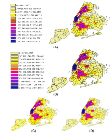
is shown in Figure 8A–8D. Figure  8D, showing weekend crime in San Francisco, does feature an additional blue patch in the top right part of the map not seen in the weekday map (Figure  8C); thus, there is some shift in spatial patterns. Interestingly, this change on the weekend mostly occurs at night (22:00–5:00), as can be seen by comparing Figure 8B and 8D. Similar trends are visible in the New York maps shown in Figure 9A–9D. All crime events that happened be-tween 5:00 and 22:00 are contained in the daytime density

maps, while those happened between 22:00 and 5:00 are con-tained in the nighttime density maps. (A similar analysis is done in [22].) Street lights may also play a role in outdoor crime events that take place from 19:00 to 5:00. The influ-ence of street lights is investigated in [23] and [24], but is not considered in the present work.

3.5

|

Model for crime prediction

Consider a spatiotemporal dataset D of crime history events for a particular city/country, with feature set F = {f₁, f2, . . . , fn}

and class labels C representing crime categories. The objec-tive is to achieve more accurate crime prediction for each category in C, minimizing classification errors and clearly indicating the confidence of each prediction. In our classifi-cation-based crime-prediction model, we refer to the set of regions (potentially including census tracts, districts, or, in the case of the GridIntersect approach, grid blocks) in the area under study as R and the time interval (the time period for which all crime events are collected together in an instance in the crime matrix) as T. Crime datasets from San Francisco and New York City are preprocessed to have the same at-tributes: Month, Day, DayOfWeek, Hour, Minute, Region

FIGURE 4 Polygon density spatial analysis of crime events at

zip-code level 0.000 0.0001–18.06 18.07–24.34 24.35–38.31 38.32–53.31 53.32–82.68 82.69–117.1 117.2–138.5 138.6–177.4 177.5–260.1 260.2–358.2 358.3–571.3

FIGURE 5 Polygon density spatial analysis of crime events at

district level RICHMOND PARK MISSION NORTHERN CENTRAL BAYVIEW INGLESIDE TARAVAL SOUTHERN * *TENDERLOIN 2.532 2.533–3.649 3.650–4.435 4.436–4.671 4.672–7.506 7.507–16.71 16.72–16.93 16.94–24.07 24.08–25.03 25.04–116.4

FIGURE 6 Variation of Z-Score for incremental spatial

auto-correlation 130 120 110 100 90 80 70 800 1120 1440 1760 2080 2400 2720 3040 3060 3680 Distance (meters) Z-scor e

FIGURE 7 Getis-Ord Hotspot analysis of crime events in San

Francisco Cold spot-99% confidence Cold spot-95% confidence Cold spot-90% confidence Not significant Hot spot-90% confidence Hot spot-95% confidence Hot spot-99% confidence

FIGURE 3 Polygon density spatial analysis of crime events at

census tract level 3.313–126.4 126.5–182.2 182.3–243.5 243.6–290.2 290.3–324.7 324.8–410.7 410.8–511.9 512.0–703.3 703.4–959.0 959.1–1354 1355–2425 2426–11620

(District in case of San Francisco and BORO_NM (Name of the borough in which the incident occurred) in case of New York), Crime Category, X (latitude), and Y (longitude). All the instances in both datasets are arranged chronologically.

The proposed crime-prediction model using spatiotempo-ral analysis consists of two main phases: crime hotspot iden-tification and crime prediction.

3.5.1

|

PHASE I: Crime hotspot

identification

Given a spatiotemporal dataset D containing the location (X,

Y), time, and date of each event (and possibly other features),

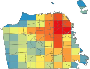
we seek to identify the regions of the study map where the concentration of crime is highest. To accomplish this task, two-dimensional hotspot analysis is conducted. The pro-posed grid-based approach, termed the HotBlock approach, consists of dividing the map into quads according to a grid that best fits the map. The grid used in this study is a square

grid Gnxn, as shown in Figure 10.

In Algorithm 1, I is the set of instances in the dataset D. Every instance contains a set of features F, including the latitude

and longitude. Block is the set of grid blocks that are identified by the GridIntersect approach (described in the next paragraph),

and CountCj

Block_b is the count of the number of crime incidences

of category Cj that belong to grid block Blockb. Count is the set

of all counts for all grid blocks and crime categories.

The GridIntersect approach first simply fits a grid onto the area under study. The extreme coordinates, that is the maxi-mum values of X and Y in the study area, are calculated, and a polygon is formed. This polygon can be divided into grid blocks according to a predefined number of rows and columns or based on a block size given in forming the grid. In this work, a square grid is used, with grid blocks of variable sizes. The objective of Algorithm 1 is to calculate the number of instances of a particular category of crime that belong to each grid block. However, the GridIntersect approach will not always yield the same size grid blocks, as is clear from Figure 10. Some grid blocks which are near the boundary of the study area may have less area than those that lie completely inside the study area.

Algorithm 2 finds AvgCountCj, the average number of

in-stances that belong to each grid block for a particular category

of crime Cj. This algorithm is used to discover a local threshold

for the existence of a particular category of crime Cj across the

given time interval T in region/grid block Blockb. Thus, there

will be a separate local threshold for each category of crime. Instead of taking the exact average value to be the threshold,

FIGURE 8 Crime-density map of San Francisco: (A) Daytime,

(B) Nighttime, (C) Weekday, and (D) Weekend 0–431 701.8991 431 701.8992–4 005 530.11 4 005 530.111–7 579 358.321 7 579 358.322–11 153 186.53 11 153 186.54–14 727 014.74 14 727 014.75–18 300 842.95 18 300 842.96–21 874 671.17 21 874 671.18–25 448 499.38 25 448 499.39–29 022 327.59 29 022 327.6–32 596 155.8 32 596 155.81–36 169 984.01 36 169 984.02–120 408 168 0–137187.5207 2 421 595.153–3 563 798.967 3 563 798.968–4 706 002.782 4 706 002.783–5 848 206.598 5 848 206.599–6 990 410.413 6 990 410.414–8 132 614.229 8 132 614.23–9 274 818.044 9 274 818.045–10 417 021.86 10 417 021.87–11 559 225.67 11 559 225.68–36 857 044 1 279 391.337–2 421 595.152 137 187.5208–1 279 391.336 (A) (B)

(C) (D) FIGURE 9 Crime-density map of New York City: (A) Daytime, (B) Nighttime, (C) Weekday, and (D) Weekend

0–299 415.9875 299 415.9876–605 771.0665 605 771.0666–912 126.1456 912 126.1457–1 218 481.225 1 218 481.226–1 524 836.304 1 524 836.305–1 831 191.383 1 831 191.384–2 137 546.462 2 137 546.463–2 443 901.541 2 443 901.542–2 750 256.62 2 750 256.621–3 056 611.699 3 056 611.7–3 362 966.778 3 362 966.779–7 483 781.5 0–107 191.1745 107 191.1746–226 129.4002 226 129.4003–345 067.6258 345 067.6259–464 005.8514 464 005.8515–582 944.0771 582 944.0772–701 882.3027 701 882.3028–820 820.5284 820 820.5285–939 758.754 939 758.7541–1 058 696.98 1 058 696.981–1 177 635.205 1 177 635.206–1 296 573.431 1 296 573.432–2 574 258.75 (A) (B) (C) (D)

some fraction of it is considered. This fraction is governed by the variable margin. In this work, after performing several ex-periments, we assigned margin the value 0.9. An additional attri-bute in the dataset gives information about whether a grid block is a HotBlock, that is, whether it contains an exceptional num-ber of crime events in all categories. HotCount, the threshold

for declaring a grid block to be a HotBlock, is calculated in Algorithm 3. Algorithm 4 is used for actual identification of HotBlocks in the study area. In this algorithm, the variable Threshold is simply the ratio of HotCount and Max(Area).

P(Cj), the probability of a particular category Cj of crime

occurring, is given by,

where |I| is the number of instances in all categories. E_Block

b, the

expectation of block Blockb, is given by,

Then, and (1) P(C_j)=Count Cj |I| , (2) E(Blockb ) = | C | ∑ j = 1 CountCj Blockb∗P ( C_j). (3) SumE_Blockb= n2 ∑ b = 1 E(Blockb ) (4) E((Blockb )2) = | C | ∑ j = 1 CountCj Blockb 2 ∗P(C_j).

FIGURE 10 Grid Intersection Map for San Francisco

Algorithm 1 BlockInstanceCount algorithm

Algorithm 2 Estimation of AvgCount (the average

number of crime instances per block per category) for HotBlock algorithm

Algorithm 4 HotBlock identification algorithm

Algorithm 3 Algorithm for estimation of HotCount,

Similarly,

Then, the standard deviation, variance, and HotCount are as in Algorithm 3.

3.5.2

|

PHASE II:

Crime-prediction approach

In the final phase of the proposed model, a training dataset is prepared from the phase I results and used provide crime predictions. In this work, the crime-prediction model uses state-of-the-art classifiers as base learners. Classification approaches have been used earlier to predict crime at a particular location [25]. Here, proposed models are based on both binary and multiclass classification based on the type of evaluation. For example, Tables 3–9 hold results for models based on multiclass classification, while in Table 10 binary classification models for mentioned cat-egories are trained and tested. The rest of the results are for multiclass classification models. Various state-of-the-art crime-prediction techniques—Naive Bayes, Decision

Tree (REPTree), and ensemble learning approaches such as bagging, voting, and stacking—are tested, with and

with-out hotspot analysis.

4

|

RESULTS AND DISCUSSION

4.1

|

Performance parameters

4.1.1

|

Standard evaluation metrics

In this work, standard metrics are used for evaluating the

pro-posed model: accuracy, true-positive rate (TPrate),

false-pos-itive rate (FPrate), precision, receiver operating characteristic

(ROC), precision-recall curve (PRC), and F1 score.

For better and more reliable predictions, a model should

have high accuracy, high TPrate, low FPrate, high precision,

and a high F1-Score. The ROC curve is a graph of TPrate as

a function of FPrate. In this work, the area under this curve is

called the ROC value; a large ROC value indicates that the model is capable of distinguishing between classes. The PRC shows the tradeoff between precision and recall for differ-ent thresholds; a large area under this curve indicates both high recall and high precision, where high precision relates to a low false-positive rate, and high recall relates to a low false-negative rate. (5) SumE_Block2 b = n2 ∑ b = 1 E((Blockb )2) .

TABLE 3 Accuracy of classification approaches to San Francisco

dataset with various grid sizes

Approach 3 × 3 4 × 4 5 × 5 6 × 6 NB 79.06 74.57 75.71 67.79 NB-k 72.09 76.27 77.14 62.71 REPTree 72.09 69.49 65.71 59.32 Bagging (NB) 76.74 74.57 72.85 64.40 Bagging (NB-k) 72.09 77.96 77.14 62.71 Bagging (REPTree) 76.74 79.66 72.85 54.23 Vote (NB) 79.06 74.57 75.71 67.79 Vote (NB-k) 72.09 76.27 77.14 62.71 Vote (NB + REPTree) 76.74 71.18 70.00 62.71 Vote (REPTree) 72.09 69.49 65.71 59.32 Stacking (NB) 79.06 76.27 75.71 50.84 Stacking (REPTree) 60.46 69.49 65.71 62.71 Stacking (NB + REPTree, meta = NB) 81.39 67.79 68.57 47.45 Stacking (NB + REPTree, meta = REPTree) 69.76 71.18 67.14 62.71

Bold values in Tables represent the best value of performance metric for the corresponding classifier.

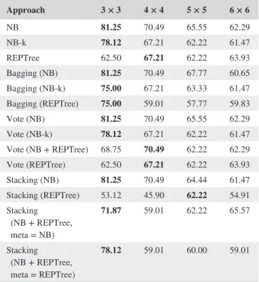
TABLE 4 Accuracy of classification approaches to New York

City dataset with various grid sizes

Approach 3 × 3 4 × 4 5 × 5 6 × 6 NB 81.25 70.49 65.55 62.29 NB-k 78.12 67.21 62.22 61.47 REPTree 62.50 67.21 62.22 63.93 Bagging (NB) 81.25 70.49 67.77 60.65 Bagging (NB-k) 75.00 67.21 63.33 61.47 Bagging (REPTree) 75.00 59.01 57.77 59.83 Vote (NB) 81.25 70.49 65.55 62.29 Vote (NB-k) 78.12 67.21 62.22 61.47 Vote (NB + REPTree) 68.75 70.49 62.22 62.29 Vote (REPTree) 62.50 67.21 62.22 63.93 Stacking (NB) 81.25 70.49 64.44 61.47 Stacking (REPTree) 53.12 45.90 62.22 54.91 Stacking (NB + REPTree, meta = NB) 71.87 59.01 62.22 65.57 Stacking (NB + REPTree, meta = REPTree) 78.12 59.01 60.00 59.01

Bold values in Tables represent the best value of performance metric for the corresponding classifier.

4.1.2

|

Confidence score

The confidence score is an indicator of the strength of the predictions made by the model. This score is derived from the hotspot identification phase. If a test instance is located in the hotspot region, the confidence score will be high; other-wise, it will be low. It is calculated as follows:

Here, CountCj

Blockb is the number of crime incidences of

cate-gory Cj that belong to block Blockb and AvgCountCj is obtained

from Algorithm 2. The confidence score will be positive for all those grid blocks that have more crime events than HotCount and negative for the rest. When CS < 0, a large absolute value indicates that the grid block has very few crime events.

4.2

|

Crime prediction using state of

art techniques

The last phase of the crime-prediction model is prediction using state-of-the-art techniques. In this phase, each classifier is trained with 60% of the data and rest are used for testing. The dataset which is given as input is obtained from phase I. The predictions are made both with and without hotspot analysis.

CSCj Block_b= CountCj Blockb−AvgCount Cj deviation .

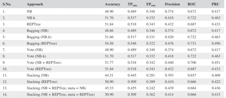
TABLE 5 Evaluation metrics for classification approaches on San Francisco dataset without hotspot analysis

S.No. Approach Accuracy TPrate FPrate Precision ROC PRC

1. NB 48.90 0.489 0.348 0.374 0.672 0.417 2. NB-k 51.70 0.517 0.332 0.418 0.722 0.463 3. REPTree 51.84 0.518 0.343 0.432 0.687 0.433 4. Bagging (NB) 48.86 0.489 0.346 0.374 0.672 0.417 5. Bagging (NB-k) 51.66 0.517 0.331 0.420 0.722 0.463 6. Bagging (REPTree) 54.56 0.546 0.322 0.476 0.731 0.496 7. Vote (NB) 48.90 0.489 0.348 0.374 0.672 0.417 8. Vote (NB-k) 51.70 0.517 0.332 0.418 0.722 0.463 9. Vote (NB + REPTree) 51.77 0.518 0.342 0.440 0.706 0.451 10. Vote (REPTree) 51.84 0.518 0.343 0.432 0.687 0.433 11. Stacking (NB) 44.51 0.445 0.281 0.393 0.657 0.408 12. Stacking (REPTree) 50.90 0.509 0.389 0.410 0.666 0.422

13. Stacking (NB + REPTree, meta = NB) 45.53 0.455 0.242 0.439 0.684 0.436

14. Stacking (NB + REPTree, meta = REPTree) 50.90 0.509 0.362 0.414 0.666 0.415

TABLE 6 Evaluation metrics for classification approaches on San Francisco dataset with hotspot analysis for optimal grid size

Approach Accuracy TPrate FPrate Precision ROC PRC

NB 79.06 0.791 0.259 0.790 0.842 0.848 NB-k 72.09 0.721 0.345 0.717 0.862 0.866 REPTree 72.09 0.721 0.264 0.739 0.745 0.724 Bagging (NB) 76.74 0.767 0.295 0.768 0.814 0.824 Bagging (NB-k) 72.09 0.721 0.345 0.717 0.851 0.854 Bagging (REPTree) 76.74 0.767 0.213 0.786 0.835 0.851 Vote (NB) 79.06 0.791 0.259 0.790 0.842 0.848 Vote (NB-k) 72.09 0.721 0.345 0.717 0.862 0.866 Vote (NB + REPTree) 76.74 0.767 0.274 0.765 0.835 0.844 Vote (REPTree) 72.09 0.721 0.264 0.739 0.745 0.723 Stacking (NB) 79.06 0.791 0.279 0.798 0.844 0.782 Stacking (REPTree) 60.46 0.605 0.405 0.466 0.500 0.522

Stacking (NB + REPTree, meta = NB) 81.39 0.814 0.183 0.820 0.896 0.902

It is found that there is a considerable improvement in the ac-curacy when hotspot analysis is used. After the testing phase, a confidence score is calculated for each of the instances using the formula defined in Section 4. Clearly, if the predicted loca-tion is in a hotspot, confidence in the predicloca-tion will be higher. The present model is entirely based on the HotBlock proach. As discussed in previous sections, there are many ap-proaches to finding dense spatial patterns of crime in a study area. The resolution level of the spatial analysis plays a very important role in identifying these dense patterns, because, at a finer resolution, a spatial unit might be identified as a hotspot, but, at a coarser resolution, the area containing it might not be.

The variation in hotspots with spatial resolution is illustrated by comparing zip-code level results (Figure 5) with district level ones (Figure 6). For this reason, the HotBlock approach of di-viding the map into equal size blocks (except those which lie around boundaries) has been selected. The grid size is varied to find an optimal size yielding the best classification results. Finally, this optimal-sized grid is superimposed on the study area using GridIntersect, as discussed in the previous section. HotBlocks are identified using Algorithm 4. It is clear from Tables 3 and 4 that the 3 × 3 grid size yields the best classi-fication results for both the datasets. The model's predictions with and without hotspot analysis using the optimal grid have

TABLE 7 Evaluation metrics for classification approaches on New York City dataset without hotspot analysis

S.No. Approach Accuracy TPrate FPrate Precision ROC PRC

1. NB 45.15 0.452 0.354 0.388 0.647 0.424 2. NB -k 47.46 0.475 0.301 0.430 0.692 0.469 3. REPTree 47.34 0.473 0.284 0.429 0.675 0.448 4. Bagging (NB) 45.18 0.452 0.354 0.387 0.647 0.425 5. Bagging (NB -k) 47.49 0.475 0.301 0.430 0.693 0.469 6. Bagging (REPTree) 48.30 0.483 0.275 0.444 0.702 0.484 7. Vote (NB) 45.15 0.452 0.354 0.388 0.647 0.424 8. Vote (NB -k) 47.46 0.475 0.301 0.430 0.692 0.469 9. Vote (NB + REPTree) 47.31 0.473 0.312 0.420 0.687 0.463 10. Vote (REPTree) 47.34 0.473 0.284 0.429 0.675 0.448 11. Stacking (NB) 44.61 0.446 0.310 0.342 0.646 0.424 12. Stacking (REPTree) 45.88 0.459 0.316 0.396 0.661 0.433 13. Stacking (NB + REPTree, meta = NB) 46.39 0.464 0.260 0.434 0.683 0.460 14. Stacking (NB + REPTree, meta = REPTree) 45.29 0.453 0.308 0.396 0.646 0.420

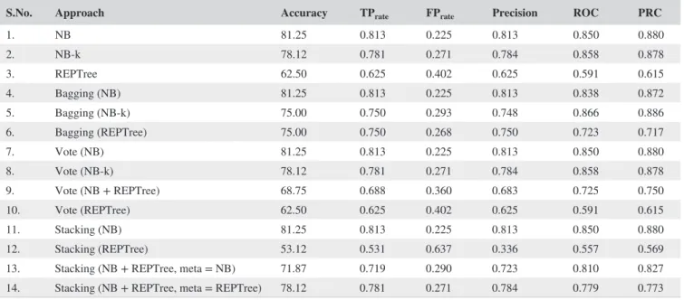
TABLE 8 Evaluation metrics for classification approaches on New York City dataset using hotspot analysis

S.No. Approach Accuracy TPrate FPrate Precision ROC PRC

1. NB 81.25 0.813 0.225 0.813 0.850 0.880 2. NB-k 78.12 0.781 0.271 0.784 0.858 0.878 3. REPTree 62.50 0.625 0.402 0.625 0.591 0.615 4. Bagging (NB) 81.25 0.813 0.225 0.813 0.838 0.872 5. Bagging (NB-k) 75.00 0.750 0.293 0.748 0.866 0.886 6. Bagging (REPTree) 75.00 0.750 0.268 0.750 0.723 0.717 7. Vote (NB) 81.25 0.813 0.225 0.813 0.850 0.880 8. Vote (NB-k) 78.12 0.781 0.271 0.784 0.858 0.878 9. Vote (NB + REPTree) 68.75 0.688 0.360 0.683 0.725 0.750 10. Vote (REPTree) 62.50 0.625 0.402 0.625 0.591 0.615 11. Stacking (NB) 81.25 0.813 0.225 0.813 0.850 0.880 12. Stacking (REPTree) 53.12 0.531 0.637 0.336 0.557 0.569

13. Stacking (NB + REPTree, meta = NB) 71.87 0.719 0.290 0.723 0.810 0.827

been compared; the model yields better performance with the HotBlock approach than with state-of-the-art approaches alone.

The results obtained for San Francisco without perform-ing hotspot analysis are shown in Table 5. The dataset has been preprocessed simply by employing Algorithm 1 and 2 and used for training and testing the crime-prediction model with different base approaches that might include a single base classifier or an ensemble of classifiers. For evaluating the performance, 60% of the data is taken as the training set and the remainder is used to test the model. The accu-racy ranges from 44.51 (base classifier: Stacking with Naive Bayes) to 54.56 (base classifier: Bagging with REPTree).

Performance has also been evaluated using all parameters for the optimal grid size for the map of San Francisco, as discussed earlier in this section. It can be seen from Table 6 that there is a considerable improvement in terms of accuracy and other performance parameters. The best performance is observed with Stacking with Naive Bayes and REPTree as base classifiers and Naive Bayes as meta classifier.

A similar approach has been tested for the New York dataset. Table  7 holds the results for the crime-prediction model without using hotspot analysis. Maximum accuracy is achieved by the Bagging model with Naive Bayes (using a kernel estimator) as the base classifier. However, when the same models are applied to the dataset preprocessed using hotspot analysis and optimal grid size experiments, there is considerable improvement in the accuracy. It can be seen from Table 8 that, with hotspot analysis included, the maxi-mum achieved accuracy increases to 81.25%.

The proposed crime-prediction model based on hotspot analysis is compared with the DeepCrime model for the New York dataset. For ease in comparison, the same performance parameters and dataset split are used. The training dataset contains crime events up to the kth month; the model attempts to predict the crime events of the (k + 1)th month.

The New York crime dataset is preprocessed so that each category can be handled separately. The proposed model for all the state-of-the-art classifiers is compared with the base-line (DeepCrime). An F1 score is recorded for all the experi-ments conducted for the individual categories of crime. Every model is tested for monthly datasets from August through December. It can be seen from Tables 9 and 10 that the pro-posed model outperforms the baseline model in most cases.

4.3

|

Parameter sensitivity analysis

The proposed crime-prediction model involves two impor-tant parameters: GridSize (the size of the grid) and #T (the time interval, that is, the number of timesteps [in days]). The proposed model's performance is evaluated by vary-ing each of these parameters while keepvary-ing the others fixed. It is important to analyze the robustness of the model over

TABLE 9

Crime-prediction results for New York City dataset across different categories in terms of Macro-F1 and Micro-F1

Month August September October November December Algorithm Macro-F1 Micro-F1 Macro-F1 Micro-F1 Macro-F1 Micro-F1 Macro-F1 Micro-F1 Macro-F1 Micro-F1 NB 0.654 0.664 0.666 0.674 0.695 0.702 0.708 0.715 0.701 0.706 NB -k 0.655 0.661 0.671 0.677 0.688 0.693 0.707 0.712 0.694 0.700 REPTree 0.633 0.653 0.655 0.665 0.613 0.646 0.626 0.666 0.587 0.619 Bagging (NB) 0.656 0.664 0.647 0.664 0.691 0.700 0.707 0.715 0.702 0.707 Bagging (NB -k) 0.652 0.658 0.668 0.678 0.688 0.693 0.704 0.708 0.697 0.700 Bagging (REPTree) 0.643 0.655 0.628 0.644 0.621 0.644 0.629 0.646 0.646 0.656 Voting(NB + REPTree) 0.653 0.665 0.658 0.672 0.652 0.669 0.635 0.666 0.616 0.638 Stacking (NB) 0.654 0.662 0.660 0.671 0.687 0.696 0.701 0.711 0.698 0.707 Stacking (REPTree) 0.589 0.649 0.528 0.598 0.579 0.623 0.584 0.620 0.555 0.587

Stacking (NB + REPTree, meta = NB)

0.655 0.662 0.655 0.661 0.686 0.693 0.642 0.652 0.636 0.638

Stacking (NB + REPTree, meta = REPTree)

0.636 0.669 0.617 0.657 0.582 0.624 0.623 0.659 0.686 0.694 DeepCrime 0.682 0.620 0.679 0.623 0.684 0.623 0.666 0.601 0.668 0.611

TABLE 10

Crime-prediction results for individual categories of crime in New York City dataset in terms of F1-score

Algorithm Burglary Robbery August September October November December August September October November December NB 0.668 0.657 0.615 0.675 0.711 0.598 0.605 0.644 0.627 0.538 NB -k 0.684 0.670 0.637 0.697 0.686 0.640 0.672 0.664 0.704 0.653 REPTree 0.668 0.626 0.606 0.519 0.729 0.656 0.574 0.701 0.705 0.531 Bagging (NB) 0.668 0.650 0.606 0.675 0.711 0.621 0.594 0.620 0.649 0.538 Bagging (NB -k) 0.698 0.662 0.637 0.682 0.686 0.640 0.696 0.677 0.690 0.653 Bagging (REPTree) 0.637 0.643 0.622 0.606 0.686 0.641 0.722 0.648 0.668 0.653 Voting (NB + REPTree) 0.668 0.657 0.606 0.625 0.729 0.678 0.588 0.671 0.719 0.585 Stacking (NB) 0.668 0.657 0.615 0.675 0.711 0.598 0.589 0.644 0.649 0.538 Stacking (REPTree) 0.668 0.650 0.410 0.555 0.686 0.494 0.530 0.505 0.727 0.635

Stacking (NB + REPTree, meta = NB)

0.668 0.650 0.566 0.675 0.686 0.674 0.611 0.701 0.744 0.680

Stacking (NB + REPTree, meta = REPTree)

0.668 0.657 0.615 0.675 0.711 0.631 0.547 0.505 0.727 0.584 DeepCrime 0.617 0.605 0.605 0.590 0.591 0.630 0.585 0.618 0.599 0.623 Algorithm Felony Assault Grand Larceny August September October November December August September October November December NB 0.646 0.600 0.572 0.577 0.566 0.844 0.833 0.831 0.831 0.836 NB-k 0.692 0.656 0.675 0.687 0.596 0.852 0.849 0.863 0.845 0.862 REPTree 0.603 0.644 0.620 0.548 0.566 0.741 0.761 0.727 0.731 0.706 Bagging (NB) 0.654 0.605 0.585 0.577 0.563 0.833 0.843 0.827 0.850 0.836 Bagging (NB-k) 0.648 0.643 0.632 0.642 0.555 0.846 0.849 0.845 0.839 0.814 Bagging (REPTree) 0.638 0.643 0.608 0.592 0.688 0.767 0.805 0.757 0.720 0.740 Voting (NB + REPTree) 0.616 0.644 0.652 0.582 0.566 0.741 0.761 0.827 0.743 0.723 Stacking (NB) 0.635 0.628 0.615 0.550 0.528 0.862 0.852 0.829 0.840 0.836 Stacking (REPTree) 0.551 0.603 0.616 0.548 0.646 0.741 0.761 0.727 0.693 0.772

Stacking (NB + REPTree, meta = NB)

0.628 0.604 0.675 0.598 0.528 0.847 0.849 0.857 0.840 0.836

Stacking (NB + REPTree, meta = REPTree)

0.607 0.627 0.605 0.643 0.442 0.741 0.852 0.775 0.693 0.772 DeepCrime 0.646 0.664 0.634 0.625 0.612 0.873 0.865 0.866 0.844 0.843

these parameters. All the graphs in the following parameter sensitivity-analysis section represent experiments performed by varying one parameter (either the spatial or the tempo-ral) while keeping the other fixed. Thus, the sensitivity of the model's predictions to the temporal and spatial resolution is studied in this section.

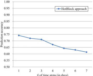
Figure 11 shows the variation of accuracy with the num-ber of time steps for all four categories under study for the New York dataset for August; Figure 12 shows the variation with grid size. Note that the accuracy value is the average of all accuracies for corresponding crime categories. It can be seen from Figures 11 and 12 that the accuracy is consid-erably better with a lower number of time steps and fewer blocks in the grid (ie, lower spatial resolution). The reason behind these results is that it is relatively easy to predict crime events in a large region for the near future but trying

to predict them a week in advance obviously diminishes the accuracy. Similarly, it is challenging to predict crime events in a very small region (a block occupying only a small frac-tion of the grid).

Figures 13 and 14 show the results of experiments per-formed on the data from San Francisco. The trend discussed in connection with the dataset from New York is observed in the dataset from San Francisco as well.

4.4

|

Spatiotemporal complexity analysis

As discussed in this work, the initial dataset D contains a set I of instances and a set F of attributes. The HotBlock approach performs spatiotemporal analysis on D and transforms it into

FIGURE 11 Temporal parameter sensitivity analysis in terms of

accuracy for New York City August dataset 0.50 0.55 0.60 0.65 0.70 0.75 0.80 0.85 0.90 0.95 1.00 1 2 3 4 5 6 7 Prediction accuracy # of time steps Burglary Robbery Felony assault Grand larceny

FIGURE 12 Spatial parameter sensitivity analysis in terms of

accuracy for New York City August dataset 0.50 0.55 0.60 0.65 0.70 0.75 0.80 0.85 0.90 0.95 1.00 3 × 3 4 × 4 5 × 5 6 × 6 Prediction accuracy Grid size HotBlock approach

FIGURE 13 Spatial parameter sensitivity analysis in terms of

accuracy for San Francisco August dataset 0.50 0.55 0.60 0.65 0.70 0.75 0.80 0.85 0.90 0.95 1.00 3 × 3 4 × 4 5 × 5 6 × 6 Prediction accuracy Grid size HotBlock approach

FIGURE 14 Temporal parameter sensitivity analysis in terms of

accuracy for San Francisco August dataset 0.50 0.55 0.60 0.65 0.70 0.75 0.80 0.85 0.90 0.95 1.00 1 2 3 4 5 6 7 Prediction accuracy

# of time steps (in days)

a new dataset D′. In this transformation, the complete set of instances I must be traversed exactly once. Every instance is a crime event. The dataset D′ is actually a three-dimensional matrix I′ × C × R. Here, I′ is the reduced set of instances de-pending on the time slot: for example, if the time slot is one day and the study time is one year, there will be 365 instances in I′. Thus, a given cell of the three-dimensional matrix D′ contains the number of crime events in a particular category that happened in a certain block in a certain period of time. Aggregation of crime events can be done in D′ depending on the type of analysis required. For example, if the number of crime events of a particular type that might happen in a given time interval is to be predicted for the entire study area, then crime events of that category in all regions will be aggregated.

5

|

CONCLUSIONS

In this work, a novel, classification-based approach to crime prediction based is proposed. Our model, HotBlock, utilizes state-of-the-art classification models but also includes some ensemble learning approaches. The HotBlock model per-forms spatiotemporal analysis of the dataset before provid-ing crime predictions. Thus, all the dynamics of crime in the real-world scenario are taken into account by the proposed model. In this work, we also seek correlations between crime rates in different crime categories and study the impact of spatiotemporal resolution on crime hotspot analysis. Also, the performance of the proposed model is tested for sensitiv-ity to variation of the spatiotemporal parameters. It is found to be robust, and any variation in the model's performance can be properly explained. The HotBlock model is compared with the baseline DeepCrime model and is found to outper-form it in most cases.

CONFLICT OF INTEREST

The authors declare no potential conflict of interests.

ORCID

Gaurav Hajela  https://orcid.org/0000-0002-9835-205X

Meenu Chawla  https://orcid.org/0000-0001-7832-8346

Akhtar Rasool  https://orcid.org/0000-0002-7759-9571

REFERENCES

1. W. Bernasco and C. Vandeviver, The geography of crime and crime

control, Appl. Geogr. 86 (2017), 220– 225.

2. X. Hu et al., Impact of climate variability and change on crime rates

in Tangshan, China, Sci. Total Environ. 609 (2017), 1041– 1048.

3. D. J. Lemon and R. Partridge, Is weather related to the number

of assaults seen at emergency departments?, Injury 48 (2017),

2438– 2442.

4. X. Zhao and J. Tang, Crime in urban areas: A data mining

perspec-tive, available at CoRR http://arxiv.org/abs/1804.08159, preprint,

2018.

5. M. R. D‘Orsogna and M. Perc, Statistical physics of crime: A

re-view, Phys. Life Rev. 12 (2015), 1– 21.

6. M. A. Andresen, Crime measures and the spatial analysis of

crim-inal activity, Br. J. Criminol. 46 (2005), 258– 285.

7. M. A. Andresen, Estimating the probability of local crime

clus-ters: The impact of immediate spatial neighbors, J. Crim. Justice

39 (2011), 394– 404.

8. L. Anselin, Local Indicators of Spatial Association— LISA, Geogr. Anal. 27 (1995), 93– 115.

9. C. Cowen, E. Louderback, and S. Roy, The role of land use and

walkability in predicting crime patterns: A spatiotemporal analysis of Miami- Dade County neighborhoods, 2007– 2015, Secur. J. 32

(2019), 264– 286.

10. D. Vildosola et al., Crime in an affluent city: Applications of risk

terrain modeling for residential and vehicle burglary in Coral Gables, Florida, 2004– 2016, Appl. Spat. Anal. Policy 13 (2019),

441– 459.

11. C. Huang et al., Deep- Crime: Attentive hierarchical recurrent

net-works for crime prediction, in Proc. ACM Int. Conf. Inf. Knowledge

Manag. (Torino, Italiy), Oct. 2018, pp. 1423– 1432.

12. M. S. Gerber, Predicting crime using Twitter and kernel density

estimation, Decis. Support Syst. 61 (2014), 115– 125.

13. L. Vomfell, W. K. Härdle, and S. Lessmann, Improving crime count

forecasts using Twitter and taxi data, Decis. Support Syst. 113

(2018), 73– 85.

14. M. L. Williams, P. Burnap, and L. Sloan, Crime sensing with Big

Data: The affordances and limitations of using open- source com-munications to estimate crime patterns, Br. J. Criminol. 57 (2016),

320– 340.

15. L. G. A. Alves, H. V. Ribeiro, and F. A. Rodrigues, Crime

predic-tion through urban metrics and statistical learning, Phys. A 505

(2018), 435– 443.

16. J. H. Ratcliffe, Geocoding crime and a first estimate of a minimum

acceptable hit rate, Int. J. Geogr. Inf. Sci. 18 (2004), 61– 72.

17. J. K. Ord and A. Getis, Local spatial autocorrelation statistics:

Distributional issues and an application, Geogr. Anal. 27 (1995),

286– 306.

18. G. N. Kouziokas, The application of artificial intelligence in

public administration for forecasting high crime risk transpor-tation areas in urban environment, Transp. Res. Procedia 24

(2017), 467– 473.

19. A. Getis and J. K. Ord, The analysis of spatial association by use of

distance statistics, Geogr. Anal. 24 (1992), 189– 206.

20. G. Mohler, Marked point process hotspot maps for homicide and gun

crime prediction in Chicago, Int. J. Forecast. 30 (2014), 491– 497.

21. K. Leong and A. Sung, A review of spatio- temporal pattern

anal-ysis approaches on crime analanal-ysis, Int. e- J. Crim. Sci. 9 (2015),

1– 33.

22. A. Rummens, W. Hardyns, and L. Pauwels, The use of

predic-tive analysis in spatiotemporal crime forecasting: Building and testing a model in an urban context, Appl. Geogr. 86 (2017),

255– 261.

23. T. Lawson, R. Rogerson, and M. Barnacle, A comparison

be-tween the cost effectiveness of CCTV and improved street lighting as a means of crime reduction, Comput. Environ. Urban Syst. 68

(2018), 17– 25.

24. Y. Xu et al., The impact of street lights on spatial- temporal patterns

of crime in Detroit, Michigan, Cities 79 (2018), 45– 52.

25. R. Iqbal et al., An experimental study of classification algorithms

AUTHOR BIOGRAPHIES

Gaurav Hajela received his Bachelor

of Engineering degree in Information Technology from Rajiv Gandhi Proudyogiki Vishwavidyalaya, Bhopal, India in 2012, and his MTech degree in Computer Science and Engineering from Maulana Azad National Institute of Technology (MANIT), Bhopal, India in 2014. Since 2015, he has been with the Department of Computer Science and Engineering, MANIT, Bhopal, India, where he is pursuing his PhD degree. His main re-search interests are Big Data analytics, machine learning, and time series prediction.

Meenu Chawla received her Bachelor

of Engineering degree in Computer Technology from MANIT, Bhopal, India in 1990, and her MTech degree in Computer Science and Engineering from Indian Institute of Technology, Kanpur, India in 1995. She received her PhD in the area of Mobile and Ad Hoc Networks (Computer Science) from MANIT in 2012. She has more than 25  years of teaching and research experience.

Currently, she is a Professor in the Department of Computer Science and Engineering at MANIT, Bhopal, India. She has published more than 50 research papers in major journals and technical conferences. Her research and teaching interests include data structure and algo-rithms, wireless communication and mobile computing, mobile ad hoc and sensor networks, cognitive radio net works, and Big Data.

Akhtar Rasool received his Bachelor

of Engineering degree in Computer Science from Rajiv Gandhi Proudyogiki Vishwavidyalaya, Bhopal, India in 2003, and his MTech degree in Computer Science and Engineering from MANIT, Bhopal, India in 2007. He received his PhD in Computer Science and Engineering from MANIT in 2014 and is presently an Assistant Professor there. He has published more than 35 research papers in international/national journals and con-ferences. His research areas include string-matching algo-rithms, parallel computing, artificial intelligence, data science, Big Data analysis, software engineering, analysis and design of algorithms, cluster and grid computing, and quantum computing.