Application of Electro-Hydraulic Proportional Valve for Steering Improvement of an Autonomous Tractor

저작자표시-변경금지 2.0 대한민국 이용자는 아래의 조건을 따르는 경우에 한하여 자유롭게 l 이 저작물을 복제, 배포, 전송, 전시, 공연 및 방송할 수 있습니다. l 이 저작물을 영리 목적으로 이용할 수 있습니다. 다음과 같은 조건을 따라야 합니다: l 귀하는, 이 저작물의 재이용이나 배포의 경우, 이 저작물에 적용된 이용허락조건 을 명확하게 나타내어야 합니다. l 저작권자로부터 별도의 허가를 받으면 이러한 조건들은 적용되지 않습니다. 저작권법에 따른 이용자의 권리는 위의 내용에 의하여 영향을 받지 않습니다. 이것은 이용허락규약(Legal Code)을 이해하기 쉽게 요약한 것입니다. Disclaimer 저작자표시. 귀하는 원저작자를 표시하여야 합니다. 변경금지. 귀하는 이 저작물을 개작, 변형 또는 가공할 수 없습니다.

Master’s Thesis of Engineering

Application of Electro-Hydraulic

Proportional Valve for Steering

Improvement of an Autonomous

Tractor

전자유압밸브를 이용한 자율 주행 트랙터

조향성능 향상 연구

August 2017

Graduate School of

Agriculture and Life Sciences

Seoul National University

Major of Biosystems Engineering

Application of Electro-Hydraulic

Proportional Valve for Steering

Improvement of an Autonomous

Tractor

Professor HAKJIN KIM

Submitting a master’s thesis of

Engineering

August 2017

Graduate School of

Agriculture and Life

Sciences

Seoul National University

Major of Biosystems Engineering

CHANGJOO LEE

Confirming the master’s thesis written by

CHANGJOO LEE

August 2017

Chair

Seong-In Cho (Seal)

Vice Chair Hak-Jin Kim (Seal)

Examiner Jung-Hun Kim (Seal)

Abstract

The most common solution to achieving automated steering in an agricultural tractor is the use of an electric motor in parallel with a conventional hydrostatic valve-based hydraulic steering system owing to its simplicity and low cost. However, the existing overlap, or dead band, of a hydrostatic valve has limited its potential benefit to automated tractor steering in terms of providing various agricultural operations, including planting and spraying, at higher speeds. The main objective of this study was to develop an electro hydraulic steering system applicable to an auto-guidance system, and to compare the performance of the developed system with a conventional automatic steering system. A proportional-feedforward control algorithm was implemented to effectively compensate the non-linear behaviors of the hydraulic cylinders used for changing the steered wheel angle of the tractor. A computer-controlled hardware-in-the-loop electro-hydraulic steering simulator consisting of two different types of valve sub-systems s, i.e., hydrostatic valve and EHPV sub-system, was designed and built for the development of the steering control algorithms and to verify the feasibility of the developed steering controller for accurate steering of the system with acceptable response times. A field test was conducted using a Real Time Kinematic GPS based autonomous tractor equipped with the developed EHPV-based steering system and an EPS-based steering system used as a control to compare and investigate their potential in enhancing the path tracking functionality of an auto-guided system. The use of the EHPV-based steering controller was shown to improve the tracking error by about 29% and 50% for straight and curved paths, respectively, as compared to the EPS-based steering system.

Keyword : Autonomous tractor, Electro-hydraulic steering valve,

Hydrostatic valve, Hardware-in-the-loop simulator, Nonlinear.

Student Number : 2015-23023

Table of Contents

Abstract ... i

Table of Contents ... ii

Chapter 1. Introduction ... 1

1.1. Study Background... 1

1.2. Description of Tractor Steering System ... 6

1.3. Automatic Steering System ... 10

1.3.1. Electric Power Steering System ... 10

1.3.2. Electro Hydraulic Steering System ... 12

1.4. Review of Literature ... 13

1.5. Research Purpose ... 16

Chapter 2. Materials and Methods ... 17

2.1. Preliminary Performance Test of Conventional Steering System ... 17

2.1.1. Purpose of Preliminary Test ... 17

2.1.2. Zero-Load Test ... 21

2.1.3. Tractor Traveling Test ... 22

2.2. Hardware-in-the Loop Simulator ... 24

2.2.1. Hydraulic Circuit ... 25

2.2.2. Hardware Description ... 27

2.3. ISO 11783 Network ... 37

2.3.1. ISO 11783 (ISOBUS) ... 37

2.4. Steering Control Algorithm ... 45

2.4.1. Dead Time ... 48

2.4.2. Dead Band ... 51

2.4.3. Static Friction ... 57

2.5. Virtual Terminal ... 61

2.6. Vehicle Traveling Test ... 66

2.6.1. Hardware Configurations ... 66

2.6.2. Trajectory Tracking Control ... 72

2.6.3. Zero-Load Test ... 74

2.6.4. Sinusoidal Tracking Test ... 75

2.6.5. Path-Tracking and Test Methods ... 76

2.6.6. Evaluation Method of Path Tracking Deviation .... 79

Chapter 3. Results and Discussion ... 81

3.1. Preliminary Test Results of EPS-based Hydrostatic Steering System ... 81

3.2. Experiment Results of Steering Behavior of Hydrostatic Steering System using HIL simulator ... 85

3.3. Experiment Results of Electrohydraulic Steering System using HIL simulator ... 81

3.3.1. Dead-Time Approximation ... 88

3.3.2. Dead-Band Compensation... 90

3.3.3. Static Friction Compensation ... 92

3.3.4. Steering Controller Test under Load Conditions ... 94

3.4. Performance Evaluation of Tractor Steering System ... 96

3.4.1. Zero Load Test ... 96

3.4.2. Sinusoidal Steering Test ... 96

3.4.3. Path-Tracking Test ... 99

Chapter 4. Conclusions

... 107

List of Tables

Table 1 Specifications of the test tractor ... 20 Table 2 Soil properties and moisture contents of test fields. ... 23 Table 3 Specifications of sensors ... 31 Table 4 Communication database for CAN. ... 43 Table 5 Hardware specifications of the navigation system ... 71

List of Figures

Fig. 1 Automatic Steering System ... 3

Fig. 2 Conventional steering system ... 7

Fig. 3 Hydrostatic steering valve... 7

Fig. 4 Rotor operation in the rotor set ... 9

Fig. 5 Photograph of Topcon electric steering system ... 11

Fig. 6 John Deere Auto Trac Universal ... 11

Fig. 7 Electro hydraulic steering valve with electrical actuation unit ... 12

Fig. 8 Schematic diagram of the steering control system ... 15

Fig. 9 System configuration of the test tractor... 19

Fig. 10 Steering angle sensor mounting position. ... 19

Fig. 11 A zero-load test to investigate the steering characteristics of the EPS-based steering system. ... 21

Fig. 12 Test fields in Suwon ... 22

Fig. 13 Soil sampling areas. ... 23

Fig. 14 Schematic view of steering system of the circuit. ... 26

Fig. 15 Photograph of the HIL simulator ... 28

Fig. 16 HIL simulator 3D CAD model. ... 28

Fig. 17 Spool characteristic curves. ... 29

Fig. 18 Gear pump. ... 29

Fig. 19 Location of sensors in the HIL simulator ... 30

Fig. 20 Cylinder stroke versus virtual steered wheel angle. ... 31

Fig. 21 The embedded real-time processing hardware. ... 32

Fig. 22 I/O interface module... 33

Fig. 23 Power supply units. ... 33

Fig. 24 Configuration of the loader system. ... 36

Fig. 25 Hydraulic circuit of the loader system. ... 36

Fig. 26 Many ‘island’ solutions ... 38

Fig. 27 AEF ISOBUS certification label ... 38

Fig. 28 Typical ISO 11783 network ... 41

Fig. 29 Topology of the steering system ... 42

Fig. 30 Block diagram of the steering controller. ... 47

Fig. 31 Dead time element. ... 48

Fig. 32 Dead-time approximation. ... 50

Fig. 33 Definition of closed center valve. ... 51

Fig. 34 Characteristic curves of steering valve at various oil-flow rates obtained experimentally from the HIL simulator. ... 54

Fig. 35 Inverse transform of the steering valve, and curve fitting model. 54 Fig. 36 Dead-band compensation model. ... 56

Figure 37 Lubrication mechanism of sliding surfaces ... 58

Fig. 38 Flow chart of static friction compensator. ... 60

Fig. 39 A VT provides ISO 11783 systems ... 61

Fig. 40 Screenshot of the Projektor Tool software. ... 63

Fig. 41 Screenshot of programming language. ... 63

Fig. 42 The auto steering status tab of the VT ... 64

Fig. 43 The positioning status tab of the VT ... 65

Fig. 44 Schematic view of steering system of the circuit ... 67

Fig. 45 Photograph of the EHPV and directional valve mounting position.68 Fig. 46 Control box installation and configuration. ... 68

Fig. 47 Photograph of the VT mounting location. ... 69

Fig. 48 Configuration of the path-tracking system ... 70

Fig. 49 Photograph of RTK base station. ... 71

Fig. 50 bicycle model description ... 72

Fig. 51 Zero-load test conducted to calibrate and measure the performance of the EHPV-based steering system. ... 74

Fig. 52 Photograph of sinusoidal tracking test. ... 75

Fig. 53 Overhead view of experiment trajectory. ... 77

Fig. 54 Photograph of path tracking test. ... 78

Fig. 55 Transformation of relative coordinates. ... 79

Fig. 56 Graphical visualization of the tracking error concept. ... 80

Fig. 57 10° step response and load variation of vehicle with EPS-based steering system. ... 82

Fig. 58 Load magnitude according to the traveling speed. ... 83

Fig. 59 Relationship between the steering wheel angle and cylinder displacement. ... 85

Fig. 60 Results of pressure and displacement of the steering cylinder based on the steering wheel angle. ... 87

Fig. 61 Sinusoidal test used for comparing the control algorithm with and without a dead-time compensator (DT). ... 89

Fig. 62 Control signal history with and without dead-time compensation (DT). ... 89

Fig. 63 Sinusoidal test used for comparing the control algorithm with and without a dead-band compensator (DB). ... 91

Fig. 64 Control signal history with and without dead-band compensator (DT). ... 91

Fig. 65 Sinusoidal test used for comparing the control algorithm with and without a static friction compensator (SF). ... 93

Fig. 66 Control signal history with and without static friction compensator (SF). ... 93

Fig. 67 Results of the steering controller implemented on the HIL simulator ... 95

Fig. 68 Comparison of experimental 10° step response times of the tractor when using the EPS- and EHPV-based steering systems under no-load conditions. ... 96

Fig. 69 Comparison of sinusoidal test using the EPS- and EHPV-based steering systems. ... 98

Fig. 70 Overhead view of experiment trajectory (Test 1). ... 100 Fig. 71 Time history of steered wheel angle along the target angle. ... 101 Fig. 72 Bar graph showing the RMS tracking and angle errors for Test 1. ... 102

Fig. 73 Overhead view of experiment trajectory (Test 2). ... 104 Fig. 74 Time history of steered wheel angle along with the target angle. 105 Fig. 75 Bar graph showing the RMS tracking and angle errors for Test 2. ... 106

Nomenclature

𝑨𝑨𝒏𝒏 flow section area (mm2)

𝑨𝑨𝒑𝒑𝒑𝒑 orifice area of the load control valve (m2)

𝑨𝑨𝒑𝒑 cylinder area of the load cylinder (m2)

𝐜𝐜(𝐬𝐬) curvature of path 𝐂𝐂 at that point (m-1₎

𝐂𝐂 path to be followed

𝑪𝑪𝒅𝒅 valve orifice coefficient

𝐝𝐝 impulse duration (ms)

𝒅𝒅𝒉𝒉 hydraulic diameter (mm)

𝒇𝒇𝑷𝑷(𝐮𝐮) nonlinear gain function of the E/H steering system

𝑮𝑮𝑷𝑷(𝐬𝐬) open-loop transfer function

𝑮𝑮𝒍𝒍(𝐬𝐬) linear transfer function

𝐈𝐈 impulse amplitude

𝒌𝒌𝟏𝟏, 𝒌𝒌𝟐𝟐 constant values

𝐋𝐋 vehicle wheelbase (m)

𝐌𝐌 point on 𝐂𝐂 which is the closest to 𝐎𝐎

𝐎𝐎 center of the vehicle virtual rear wheel

𝚫𝚫𝐏𝐏 pressure drop across an orifice (N/m2₎

𝒒𝒒𝒊𝒊 input (target angle, θr) variable of physical system (°)

𝒒𝒒𝒐𝒐 output (steered wheel angle, θy) variable of physical (°) system (°)

𝐐𝐐 flow rate (L/min)

𝑸𝑸𝒊𝒊, 𝑸𝑸𝒐𝒐 Laplace transform of the time functions 𝒒𝒒𝒊𝒊 and 𝒒𝒒𝒐𝒐

𝑸𝑸𝒑𝒑 flow rate across the load control valve (m3/s)

𝑹𝑹𝒙𝒙(𝒏𝒏), 𝑹𝑹𝒚𝒚(𝒏𝒏) reference path (m)

𝐏𝐏 pressure in both chambers of the steering cylinder (Pa)

𝐬𝐬 curvilinear abscissa of point 𝐌𝐌 along 𝐂𝐂

𝒕𝒕𝟎𝟎 time when the threshold value is exceeded (s)

𝐯𝐯 tractor linear velocity at point 𝐎𝐎 (m/s)

𝒑𝒑 average flow velocity (m/s)

𝐕𝐕 piston speed (m/s)

𝒙𝒙𝒄𝒄, 𝒚𝒚𝒄𝒄 center of turning path (m)

𝒙𝒙𝒈𝒈, 𝒚𝒚𝒈𝒈 current tractor position (m)

𝐲𝐲 lateral deviation of the tractor with respect to 𝐂𝐂 (m)

𝒚𝒚̇ velocity of steering actuator (m/s)

𝛌𝛌 viscosity-temperature coefficient

𝜼𝜼 dynamic viscosity at reference temperature θ (℃) (kg/m·s)

𝜼𝜼𝟎𝟎 dynamic viscosity at reference temperature θ0 (℃) (kg/m·s)

𝜽𝜽� angular deviation of the vehicle (°)

𝜽𝜽𝒄𝒄(𝒔𝒔) orientation of the tangent to 𝐂𝐂 at that point (°)

𝜽𝜽𝒕𝒕 orientation of the tractor centerline (°)

𝝉𝝉𝑫𝑫𝑫𝑫, dead-time value (ms)

𝛅𝛅 orientation of the front wheel with respect to tractor centerline (°)

𝛒𝛒 fluid mass density (kg/m3₎

Chapter 1. Introduction

1.1. Study Background

Most agricultural field operations are performed using parallel swathing or switchback operation. Each subsequent pass across the field should be parallel to the previous and separated by a distance equal to the treatment width of the implement. This kind of operation is very repetitive and can become monotonous for the operator

(Stombaugh, T., 1997).

Automatic steering technology is a revolutionary invention in agricultural machinery that completely changed the way farm. This technology is currently being used very effectively for planting, spraying, and harvesting of row crops. It can lower costs and increase profits by improving efficiency and productivity of farm operations. Auto-guidance systems have the capability to steer a vehicle across the field in a straight line or any predetermined track (Ehsani. R., and E. Ontermaa, 2011).

In agriculture, accurate vehicle steering is an important objective. Auto-guidance systems can potentially steer a vehicle more precisely than can a human operator, such as tilling, planting, spraying,

fertilizing, harvesting and other farming operations. 1

Tractor implements are guided through accurately-spaced passes or swaths, the spacing of which is determined by the swath width of the equipment. However, gaps and overlaps can occur when operators deviate from the ideal guide paths, resulting in under-coverage and over coverage respectively. Such gaps and overlaps are detrimental to agricultural operations and can reduce crop yields. For example, gaps in coverage reduce the effective areas of yields being cultivated and treated. Overall crop production may suffer as a result. Overlaps in coverage tend to be inefficient and wasteful of materials, such as fertilizer, pesticides, herbicides, seed, etc. Another potential problem with overlapping coverage relates to the potential crop-damaging effects of double applications of certain agricultural chemicals.

Conventional steering system used in construction and agricultural machines alike is a so-called hydrostatic steering system. The vehicles have traditionally utilized a full fluid-linked steering system in which turning the steering wheel rotates the hydrostatic valve which is mechanically coupled to the steering shaft and opens a control port which releases flow of hydraulic fluid to the steering cylinder.

The most common solution to active steering for auto-guidance systems is a combination of an electric motor in parallel with the

hydraulic system, which is a simple, less expensive and easily

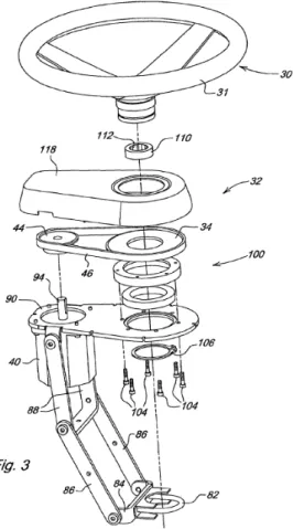
installed the steering system that minimizes or eliminates substantial steering system modifications (Amico, A. D., 2016). The present invention shown in Fig. 1 relates to automatic steering systems for vehicles. Nelson et al (2006) developed structure for converting a conventional steering system of an off-road vehicle to automatic steering system.

Fig. 1 Automatic Steering System (U. S. Patent 7,349,779 B2). A motor 40 mounted on the end of the steering shaft 20 to provide direct drive to the shaft

20 at a location offset from hand grip portion 30.

However, such a motor-based steering system has some

disadvantages. First, on account of the necessarily existing overlap of the hydrostatic valve for a control port, hydrostatic steering has a

relatively high steering play of up to ±5°. Further, there is a dead

time between the start of steering wheel movement and the steering cylinder movement. Second, the design is relatively elaborate because, on account of the relatively long distance between the steering wheel, steering shaft and the axle where the steering cylinder is located, correspondingly long hydraulic pipes have to be installed. This, when added to the amount of the above-mentioned steering play, creates a dynamic behavior which is difficult to influence given the nature of the hydraulic circuitry and the hydraulic components used.

Optimization can be obtained only with difficulty by adjustment of the hydraulic components. The dynamic behavior is such that it is difficult to drive exactly straight ahead, which at relatively high traveling speeds places high demands on control abilities (Diekhans, 2000).

Since the purpose of this study is to improve the performance of conventional steering systems, a possible solution would be to use electro-hydraulic proportional valve (EHPV). These are actuated by a solenoid, thereby providing an electronic interface. An

electrohydraulic solution takes advantage of the high power density from fluid power systems, which gives a very compact solution (Amico, A. D., 2016).

1.2. Description of Tractor Steering System

The power required when steering a tractor is very high compared to a passenger car. This becomes obvious when considering the relative difference in front axle load. The tractors have traditionally utilized a full fluid-linked steering system, and the most common front axle steering arrangement for a hydraulic steering cylinder. Because of their high power density in comparison to its volume, hydraulic drives are qualified for the use in vehicles with high steering loads.

The different parts of a conventionally steered front axle on a tractor are shown in Fig. 2. The steering hydrostatic valve shown in Fig. 3 is connected to the steering wheel and to both ends of the piston-and-cylinder steering unit by hydraulic lines. The hydrostatic valve, usually of the rotor type, performs both the operation of supplying the operating fluid to the power cylinders for steering the wheels and the metering of the fluid required to perform the steering operation. This type of hydraulic steering system is satisfactory for conventional tractors, trucks and earth moving equipment.

Fig. 2 Conventional steering system (Source: Danfoss).

Fig. 3 Hydrostatic steering valve (Source: Danfoss).

In hydraulic steering systems for land vehicles, the most commonly used form of valve for use in power-assisted steering mechanisms is a hydrostatic valve. The hydrostatic valve includes a valve arrangement including a spool that extends through a sleeve. The spool and the sleeve are coaxially aligned along an axis, and a limited range of relative rotational movement about the axis is

permitted between the spool and the sleeve. The valve arrangement is normally biased toward a neutral state. The valve arrangement is displaced from the neutral state to an operating state by rotation of a steering wheel coupled to the spool. When the valve arrangement is in the operating state, pressurized fluid flows through the valve

arrangement and into a fluid pressure actuated a rotor, thereby releasing the flow of hydraulic fluid to the steering cylinder.

Each lobe of the rotor has a diametrically opposite lobe, when one lobe is in a cavity its opposite lobe is at the crest of the stator’s convex form opposite the cavity (Fig. 4). As the rotor is rotated, each lobe in sequence is moved out of its cavity to the crest of stator’s convex form and this forces each opposite lobe, in sequence, into a cavity.

Fig. 4 Rotor operation in the rotor set (Source: Parker Hydraulics)

Operating state means a state where sufficient pressurized flow passes through the valve arrangement to drive movement of the rotor displacement mechanism. There has generally been excessive “neutral dead band” because of steering wheel can reverse direction with little or no resistance. When relative rotation is first generated between the spool valve and the valve sleeve, the valve arrangement initially

passes through the dead band, typically ±5°degree or so, where

insufficient flow passes through the valve arrangement to drive the displacement mechanism. Once the valve arrangement rotates past the dead zone, the valve arrangement is in the operating state where sufficient flow passes through the valve arrangement to drive

movement. However, such that the steering control at relatively higher vehicles speeds is unacceptable because there is a time delay between the start of steering wheel movement and the steering cylinder

movement.

1.3. Automatic Steering System

1.3.1. Electric Power Steering System

A change of hydraulic systems to solely electrically operated steering systems (Electric Power Steering, EPS) has taken place in passenger car steering systems during the last years. The use of these systems was originally limited to small vehicles because the power density of the electronic parts and the energy available from the on-board wiring was not sufficient to serve bigger vehicles and higher steering powers (Harrer, M., and P. Pfeffer. 2015).

Active steering is referred to as the possibility to control the output torque required to turn the wheels or manipulate the steering angle with an electronic signal. The most common solution to active steering for tractors is a combination of an electric motor and the hydraulic system. There are universal steering systems available as retrofit solutions. In this case, an electric motor is either frictionally or force-fit engaged to the steering column. There is no direct interaction with steering hydraulics. Examples of those retrofit solutions are John Deere Auto Trac Universal, Topcon electric steering system and Trimble EZ-steer (Winner, H., S. Hakuli, F. Lotz and C. Singer, 2015, Fig. 5, 6).

Fig. 5 Photograph of Topcon electric steering system

Fig. 6 John Deere Auto Trac Universal

1.3.2.

Electro Hydraulic Steering System

Electro-hydraulic (E/H) steering systems are being developed for heavy-duty industrial machines because of their potential versatility over mechanical and hydraulic steering systems. Its relatively high power-to-weight ratio and electronic controls provide effective means of power transmission. However, including load dependent dead-band, asymmetric flow gain, hysteresis, saturation, and time delay, results in difficulties in designing high performance steering systems.

A basic system consists of a pilot steering unit as the signal source and an electro hydraulic steering valve block which controls oil flow to the steering cylinders proportional to the pilot flow. The system can be extended to include an electrical actuator so that, as an alternative, it becomes possible to steer with a joystick

Fig. 7 Electro hydraulic steering valve with electrical actuation unit (Source: Danfoss).

1.4. Review of Literature

Electro-Hydraulic Steering Controller

Zhang et al. (2000) designed an E/H steering system for off-road vehicles. Their E/H system exhibits nonlinear behaviors, limiting the use of computer simulations to investigate its system dynamics. A hardware-in-the-loop (HIL) E/H steering simulator was developed to improve the efficiency in researching the E/H steering dynamics. With an appropriate orifice opening control, the simulator is able to

simulate the desired load applied to the system.

E/H systems are highly linear with a large dead band, non-linear flow gain, and saturation. Conventional control technologies such as a proportional-integral-derivate (PID) controller have limitations in providing satisfactory steering control for off-road vehicles. Qiu et al. (2001) designed an FPID controller to provide satisfactory steering control. Their FPID controller consists of a feedforward loop and a PID loop. The feedforward loop was designed to compensate for the dead band and saturation inherent to an E/H steering system, and an inverse valve transform was adopted to determine the appropriate degree of valve opening. Furthermore, to overcome the static friction, an impulse excitation signal generator was used.

Zhang. (2003) developed a generic fuzzy controller applicable to a hydraulic cylinder owing to its ability to compensate for non-linearity of the system. A hierarchical control rule derivative technique was developed to create the control rules for the generic controller.

Jiang. (2009) developed a PID-based steering controller using an E/H valve. Through step-response tests, the PID-based algorithm was shown to work well under different external load forces. However, the flow rate affects the control precision of the steering controller, and a corresponding PID value is used to accurately control the cylinder position. An additional model is needed to compensate for the flow rate.

Lenain et al. (2006) designed a model prediction control for compensate actuator delays, which is adapted to the control law with incorporated sliding control and enables both anticipation of an

approaching curvature and sliding compensation. The reference path geometry and low-level model enable the anticipation of an

approaching curvature. Using such information, it is possible to send a control value to the actuator the moment before a curve appears.

Rekow et al (2007) developed a stable steering control system, which includes a hydrostatic valve coupled to the steering wheel for

generating a hydraulic signal as a function of the steering wheel positioning, an electro-hydraulic valve that generates a hydraulic signal that functions as an electronic control signal, an electronic control unit an generating the electronic control signal, and a

hydraulic unit combining the first and second hydraulic signals and supplying a hydraulic control signal to the hydraulic steering actuator. As shown in Fig. 8, a T unit (16) combines the flows from the valves (14) and (18), and supplies the combined flow to a conventional steering cylinder (20) (Fig. 8). The benefit of this system is that it naturally compensates for a dead band or hysteresis occurring in the hydro-mechanical parts of the system. The system continuously monitors and augments the stability of the vehicle.

Fig. 8 Schematic diagram of the steering control system (U. S. Patent 0256884 A1).

1.5.

Research Purpose

Little research has been reported on the performance differences between motor and spool-based steering systems. It is not clear what issues are critical to a conventional steering system. Therefore, the main objective of this study was to develop an electro hydraulic

steering system capable of being used in an auto-guidance system, and to compare the performance of the developed system with a

conventional automatic steering system.

The specific sub-objectives of this study are as follows: 1. Develop an HIL steering simulator for easier problem

detection, and encourage the development of a new steering system.

2. Analyze of the response capabilities and dynamic characteristics of the hydrostatic valve.

3. Design an electro-hydraulic steering controller capable of providing automatic steering in an agricultural vehicle. 4. Compare the performance of the steering controller with a

conventional steering system under actal field conditions.

Chapter 2. Materials and Methods

2.1.

Preliminary Performance Test of Conventional

Steering System

2.1.1. Purpose of Preliminary Test

Before starting the design of the simulator, preliminary vehicle tests were conducted to evaluate the performance of a conventional steering system and to find directions for improvement. In addition, to determine the range of load to apply to the laboratory-scaled

simulator, it was necessary to evaluate not only the steered wheel characteristics but also the steering loads on an actual tractor.

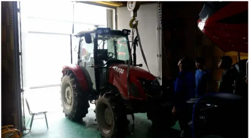
A photograph of the experiment system used in this study, a TongYang Moolsan Model TX803 tractor, is shown in Fig. 9. The tractor used an open-center hydraulic circuit equipped with a

hydrostatic steering valve. A fixed displacement gear pump driven by an engine was used to supply a constant flow to the hydrostatic valve.

An EPS (Unmanned Solution) was used in the steering column to rotate the steering wheel, and was controlled through CAN

communication. Based on the target angle determined by the EPS control module, the current from the motor drive circuit to the EPS motor was controlled to within the target amount, and the motor operated accordingly. The front wheel angle was measured using a

rotary encoder, and the sensing shaft was attached to a king pin of the wheel being monitored (Fig. 10). In addition, pressure sensors were used to measure the chamber pressure conditions and calculate the loading forces (Han, X. Z., 2013, 2017).

Fig. 9 System configuration of the test tractor. (TongYang Moolsan Model TX803 tractor)

Fig. 10 Steering angle sensor mounting position.

Table 1 Specifications of the test tractor Name Specifications Gear pump - Displacement : 9.0 cc/rev - Speed ratings : 500 ~ 3000 RPM - Max pressure : 210 kgf/cm2 Hydrostatic Steering valve - Rated Flow : 16 LPM - Displacement : 120 cc/rev

- Relief valve pressure : 145 ~ 150 kgf/cm2

- Open center

- Non load reaction type

Hydraulic steering cylinder - Cylinder stroke : 123mm - Piston diameter: 60Φ - Rod diameter: 35 Φ - Working pressure : 100kgf/cm2 - Double acting - Double rod EPS - Continuous torque : 0.52 N-m - Peak torque : 0.84 N-m

- Nominal continuous power : 204 Watt - No load Speed : 5,200 RPM

- Rotor inertia : 0.706 10-5_kg-m2

Steer sensor

- Model :ComeSys RD06001 - Steer sensor travel : 360 deg - Analogue output Pressure sensor - Model : HySense PR 110 - Range : 0 ~ 600 bar - Signal : 0 ~ 20 mA 20

2.1.2. Zero-Load Test

The forces and moments exerted on turning wheels originate from the ground’s reaction to the steering action generated at the

tire-ground interface (Mas, F. R., and Z. Qin, and A. C. H., 2010). To investigate the steered wheel characteristics in response to an applied load, steering response experiments were carried out under no load conditions, with a flow rate of around 10.5 LPM. (Zhang. Q., J. F. Reid, and D. Wu, 2000).

As shown in Fig. 11, the front wheel axle of the tractor was raised from the ground.

The EPS provided step input commands through the steering wheel, and the steered wheel angle and chamber pressures were measured at 50 Hz.

Fig. 11 A zero-load test to investigate the steering characteristics of the EPS-based steering system.

2.1.3. Tractor Traveling Test

To obtain data on the steering characteristics under an actual traveling environment, the steering response experiments were

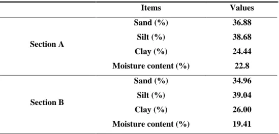
performed at constant speeds on a farm. Fig. 12 shows test location on the Seoul National University Farm in Suwon. Fig. 13 and Table 2 represents the physical properties of the soil and soil characteristics were classified as Sandy Loam according to USDA (Han, X. Z., 2017).

Fig. 12 Test fields in Suwon

Fig. 13 Soil sampling areas.

Table 2 Soil properties and moisture contents of test fields. Items Values Section A Sand (%) Silt (%) Clay (%) Moisture content (%) 36.88 38.68 24.44 22.8 Section B Sand (%) Silt (%) Clay (%) Moisture content (%) 34.96 39.04 26.00 19.41 23

2.2. Hardware-in-the Loop Simulator

Hardware-in-the-loop is the simulation technique where a part of the software implemented simulation model is replaced by actual hardware. This has the advantage of being able to test parts of the system without going for the full prototype, especially for large systems (Amico, A. D, 2016).

It is difficult to evaluate steering system properly such as steering response characteristics without actual vehicle test. But if steering system can be evaluated more accurately during the simulator which is carried out before actual vehicle testing, it will be possible to detect problems more easily and to encourage the development of a new steering system.

This section 2.2 gives an overview of the hardware involved in the HIL simulator.

2.2.1. Hydraulic Circuit

A schematic view of the steering system of a circuit is shown in Fig. 14. In this study, the conventional system is not be tampered with so that manual capability is not lost, and the electro-hydraulic steering capability to the tractor is added for system comparison.

The simulator was basically build up a full fluid-linked steering system and used the conventional open-center circuit. The hydraulic circuit has manual and automatic steering modes for selectively steering steerable wheels of the vehicle. In the manual mode, the flow is directed only toward the hydrostatic valve. When an EHPV is controlling a spool in the manual mode, a steering cylinder cannot be operated. On the other hand, in the automatic steering mode, when a directional valve is powered on, the flow passes through the EHPV and the hydrostatic valve. The directional valve is 2-way normally open solenoid directional valve from HYDAC. A loader system is designed a closed-circuit, and a detail description of a loader system follows below.

Fig. 14 Schematic view of steering system of the circuit.

2.2.2. Hardware Description

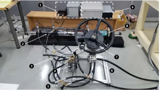
A photograph of the HIL simulator is shown in Fig. 15. As shown in Fig. 16, actuators of this HIL simulator consists of a steering cylinder and a load cylinder, which is connected in series.

The steering cylinder get their power from pressurized hydraulic fluid by the hydrostatic valve and the 4/3 EHPV respectively.

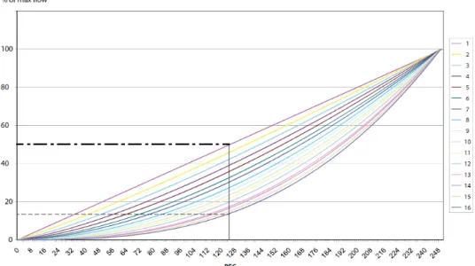
An EPS is connected through gears on the steering shaft to control the hydrostatic valve and connected to a microprocessor which is controlled via CAN communication and moves with the steering shaft. The EHPV is a hydraulic electrically controlled servo valve, PVG 32 model, from Danfoss. The EHPV built in a PVED-CC that is a digital controlled actuator for PVG 32, which is compliant to the ISOBUS standard for flow control. Fig. 17 shows spool characteristic curves of a PVED-CC, configurable range 1(linear) to 16. In this study, linear curve, default value 1, was chosen. The spool is controlled by flow commands in steps of 0.4% or by spool position with 250 positions.

A fixed displacement gear pump driven by an electric motor, which produces a maximum flow of 24.5 liters per minute, is used in the hydraulic system (Fig. 18). An AC motor inverter, iG5A model from LSIS, varied the angular speeds of the motor shaft.

Fig. 15 Photograph of the HIL simulator (○1EA: Controller & Data acquisition

units, A○2EA: Steering cylinder, A○3EA: Proportional flow control valve, A○4EA: EHPV, A○5E

A

: Directional valve, A○6EA: Hydrostatic valve, A○7EA: EPS,

A

○8EA: Load cylinder, A○9EA: Power supply units)

Fig. 16 HIL simulator 3D CAD model.

Fig. 17 Spool characteristic curves. Slope curve is a progressivity scaling of the set point.

Fig. 18 Gear pump.

A photograph of a location of sensors in the HIL simulator is shown in Fig. 19, and Table 3 shows specifications of sensors used in HIL simulator. To measure the steered wheel angle, a potentiometer is fitted on the steering cylinder. Since the steered wheel angle and the cylinder displacement has a direct relationship, the steered wheel angle values are calculated by measuring the cylinder stroke. Fig. 20 shows the relationship between cylinder displacements and steered wheel angles, which is obtained using the TX803 tractor.

Pressure sensors are used to measure the pressure each cylinder both chamber pressures, and pump pressures, and a force sensor measures the force applied by the load cylinder.

Fig. 19 Location of sensors in the HIL simulator

Table 3 Specifications of sensors Name Specifications Potentiometer - Manufacturer : MINOR - Model :KDC - Range : 0 ~ 300mm Pressure sensor - Manufacturer : VALCOM - Model : VKRQ - Range : 0 ~ 35 Mpa - Strain gage type

Force sensor - Manufacturer : Curiotec - Model : CSB-1T - Capacity : 1tf Flow sensor - Manufacturer : HYDROTECHNIK - Model : HySense QG - Range : 0.05 ~ 3000 LPM - Gearwheel type

Fig. 20 Cylinder stroke versus virtual steered wheel angle.

y = 0.4124x + 1.2304 -50 -40 -30 -20 -10 0 10 20 30 40 50 -100 -50 0 50 100 Vi rt u al S teered W h eel A n g le( d eg ) Cylinder Displacement(mm) 31

The EHPV is controlled by an embedded real-time processing hardware, VN8910A with inserted VN8950 CAN module from Vector (Fig. 21). Fig. 22 shows an I/O interface module (VT2816, Vector) that provides 12 inputs and 4 outputs for analog signals. They may be connected directly to the inputs or outputs of an ECU. The embedded real-time processing hardware runs on CANoe software and can be operated in a stand-alone mode, allowing the system operation without any additional user PC.

Fig. 21 The embedded real-time processing hardware.

CANoe software was developed to meet the essential needs of the CAN-based module or system developer by combining a

comprehensive set of measurement and simulation capabilities. CANoe can interface to multiple CAN networks (or other common small area network protocols), and provide accurate time-stamped

measurements for all communication transfers. Fig. 23 shows power supply units that convert AC power from the wall into the right kind of power for the individual parts.

Fig. 22 I/O interface module.

Fig. 23 Power supply units.

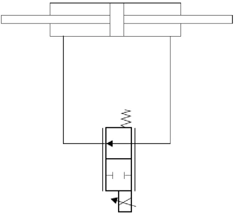
The loader system is designed to provide loads on the steering cylinder. The load cylinder is attached to generate the load

experienced by the steering system, and this system consists of a double rod, double-acting hydraulic cylinder, and a proportional flow control valve (Fig. 24). The proportional flow control valve is a normally closed, direct-acting, spring-loaded, spool type proportional flow control valve, PWK06020V model, from HYDAC.

Between the load cylinder and the steering cylinder, the force sensor measures the force applied by the load cylinder. The loader system is designed a closed-circuit flow to allow fluid movement between the chambers due to the load (Fig. 25). The load on the steering cylinder is determined by the pressure drop across the piston of the load cylinder which is controlled by the orifice area of the proportional flow control valve and the speed of the piston. The orifice area of the valve regulates the pressure drop across the valve, and therefore, provides the desired load to the system. In the

incompressible approach, the flow difference across the piston of the load cylinder is assumed to be the same as that across the flow control valve. The fluid flowing through the valve orifice is forced by the motion of the piston. The following relations formed the dynamic

model of the load simulator (Zhang. Q., J. F. Reid, and D. Wu, 2000). 𝑄𝑄𝑝𝑝 = 𝑐𝑐𝑑𝑑𝐴𝐴𝑝𝑝𝑝𝑝�2_𝜌𝜌�𝑃𝑃𝑝𝑝1− 𝑃𝑃𝑝𝑝2� (1) 𝑄𝑄𝑝𝑝 = 𝐴𝐴𝑝𝑝𝑦𝑦̇ (2) 𝐹𝐹𝑝𝑝 =𝜌𝜌𝐴𝐴𝑝𝑝 3 2𝑐𝑐_𝑑𝑑2� 𝑦𝑦̇ 𝐴𝐴𝑝𝑝𝑝𝑝� 2

𝑠𝑠𝑠𝑠𝑠𝑠𝑠𝑠

where 𝑄𝑄_𝑝𝑝 flow rate across the load control valve (m3/s), 𝐶𝐶_𝑑𝑑

valve orifice coefficient, 𝐴𝐴_{𝑝𝑝𝑝𝑝} orifice area of the load control valve

(m2_), ρ fluid mass density (kg/m3_), P pressure in both chambers of

the steering cylinder (Pa), 𝐴𝐴_𝑝𝑝 cylinder area of the load cylinder (m2_),

and 𝑦𝑦̇ velocity of steering actuator

Fig. 24 Configuration of the loader system.

Fig. 25 Hydraulic circuit of the loader system.

2.3. ISO 11783 Network

2.3.1. ISO 11783 (ISOBUS)

ISO 11783, also known as ISOBUS, is a CAN higher layer

protocol based on the SAE J1939 standard for forestry and agricultural vehicles. The primary goal of ISOBUS is to standardize the

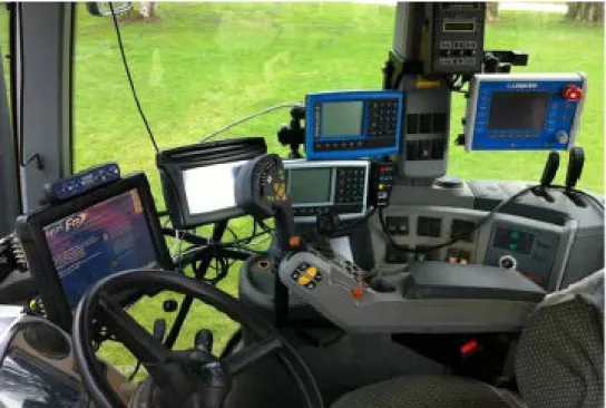
communication which takes place between tractors and implements while ensuring full compatibility of data transfer between the mobile systems and the office software used on the farm. Instead of different control boxes in the cab, ISOBUS allow the operator to use one display for an entire fleet of implements. Fig. 26 shows different control units for Non-ISOBUS implements.

ISO 11783 was a joint development by manufacturers in the agricultural and forestry industry to address the increasing needs for electronic control in the machinery and vehicles they produce. The conformance tests are performed by AEF accredited test laboratories. When a device passes the conformance tests it then receives an AEF ISOBUS Certification label which not only shows that the device conforms to ISO 11783 standard and AEF design guidelines but also the functionalities the device supports. Fig. 27 shows ISOBUS certification label.

Fig. 26 Many ‘island’ solutions to operate implements or perform other tasks

Fig. 27 AEF ISOBUS certification label

ISO 11783 supports two or more network segments. One segment is identified as the tractor network. This segment is intended to

provide the control and data communications for the drive train and chassis of the tractor or primary power unit in a system. The second segment is identified as the implement network that provides the control and data communications between implements, and between implements and the tractor or main power unit in the system. Fig. 28 illustrates the topology of a typical network in agriculture and forestry that uses serial control and communications data.

As shown in Fig. 29, in this study, a network topology of four ECUs was designed based on ISO 11783 standard: a steering ECU, an EHPV, an EPS, and a virtual terminal (VT). Table 4 shows the

communication databases between ECUs (ISO. 11783-7).

The steering ECU determines a direction and an amount of flow commands according to Target Angle message (0x600) and steered wheel angle data from the potentiometer, and Auxiliary Valve

Command message (PGN: 65072) is sent to the CAN bus. The EHPV built in a PVED-CC that is a digital controlled actuator for PVG 32, which is compliant to the ISOBUS standard for flow control. The EHPV receives Auxiliary Valve Command message via CAN bus, and

controls solenoid spool valve. The EPS receives Target Angle message (0x600) via CAN bus, and a current from the motor drive circuit to the EPS motor is controlled by PID controller within the target current amount, and the motor operates accordingly. The VT provides a capability to display information and to retrieve data from an operator. A detail description of the VT follows section 2.5.

Fig. 28 Typical ISO 11783 network

Fig. 29 Topology of the steering system

Table 4 Communication database for CAN.

1. GNSS Position Rapid Update (IEC 61162-3)

PGN 129025 DLC 8Byte

0~3Byte Latitude (Value Type: Signed, Unit: deg ) 4~7Byte Longitude (Value Type: Signed, Unit: deg )

2. Speed (IEC 61162-3)

PGN 128259 DLC 8Byte

0Byte Sid (Value Type: Unsigned)

1~2Byte Speed Water Reference (Value Type: Unsigned ) 3~4Byte Speed Ground Reference (Value Type: Unsigned, Unit: m/s )

3. Vessel Heading (IEC 611262-3)

PGN 127250 DLC 8Byte

0Byte Sid (Value Type: Unsigned)

1~2Byte Heading Sensor Reading (Value Type: Unsigned, Unit: rad ) 3~4Byte Deviation (Value Type: Signed, Unit: rad )

5~6Byte Variation (Value Type: Signed, Unit: rad ) 7Byte

56~57bit Heading Sensor Ref (Value Type: Unsigned ) 4. Attitude (IEC 61162-3)

PGN 127257 DLC 8Byte

0Byte Sid (Value Type: Unsigned ) 1~2Byte Yaw (Unit: rad ) 3~4Byte Pitch (Unit: rad ) 5~6Byte Roll (Unit: rad )

5. Target Angle (Not follow ISO 11783 standard)

ID 0x600(11bit) DLC 3Byte

0Byte Mode (01: Mode on, 00: Mode off ) 1~2Byte Target Angle (Value Type: Signed, Unit: deg ) 6. Primary Steered Wheel Angle (Not follow ISO 11783 standard)

ID 0x105(11bit) DLC 2Byte

0~1Byte Position (Value Type: Unsigned, Unit: deg ) 7. Guidance System Command (ISO 11783-7)

PGN 44288 DLC 8Byte

0~1Byte Curvature Command (Value Type: Unsigned )

2Byte bits 2~1 Steering Command Status (00: not intended for steering, _{01: intended for steering )}

2Byte

Bits 8~3 Reserved

4~7Byte Reserved

8. Auxiliary Valve Command (ISO 11783-7)

PGN 65072 DLC 8Byte

0Byte PFC (Unit: 0.4%/bit)

1Byte

Reserved

2Byte

Bits 8~7: Fail Safe Mode Bits 6~5: Reserved Bits 4~1: Valve State 3~7Byte Reserved

2.4. Steering Control Algorithm

Hydraulic control system are used in most industries where heavy objects are manipulated or large forces are exerted on their

surroundings. However, the rather complex structure of such systems makes it difficult to develop suitable, preferably low-order models of the dynamic of the plant (Jelali. M., and H. Schewarz. 1995).

Hydraulic servo systems consist of components such as servo valves, actuators and pumps whose dynamic characteristics are complex, nonlinear and time-varying. Conventional controller design based upon linearized time invariant models may not guarantee satisfactory performance due to variation of the operating point (Ziaei. K, 1998).

Nonlinearities are of particular importance in hydraulic control. In most nonlinear systems the problem is one of determining the effect on performance of certain nonlinear elements. No general nonlinear theory exists, but there are several techniques which are applicable to certain classes of problems.

This section describes the development of a steering controller for vehicles equipped with an EH steering system. An EHPV was used as an orifice valve to supply different flow rates to the steering cylinder by changing the displacement of the spool (driven by a solenoid),

according to the specified of oil flow, which ranges from 0 to 250, through the CAN bus. As shown in Equation (4), the flow across each orifice in a hydraulic valve was generally given using an orifice equation. The dynamic viscosity of a liquid varies considerably with the temperature, and thus a hydraulic fluid has a significant impact on the operation of a hydraulic system, specifically at low temperatures. The effect of temperature on the dynamic viscosity is also described through Equation (5). The discharge coefficient depends on the geometry of the conduit and on the Reynolds number which can be approximated using Equation (6).

𝑄𝑄 = 𝐶𝐶𝑑𝑑𝐴𝐴𝑛𝑛�_𝜌𝜌2∆P (4) 𝜂𝜂 = 𝜂𝜂0𝑒𝑒−𝜆𝜆(𝜃𝜃−𝜃𝜃0) (5) 𝐶𝐶𝑑𝑑 = 1 �𝜌𝜌𝑝𝑝𝑑𝑑ℎ𝑘𝑘1 𝜂𝜂 +𝑘𝑘2 (6)

where Q is the flow rate across the orifice, Cd is the discharge

coefficient which is dependent on the Reynolds number, An is the flow

section area, ρ is the oil density, ∆P is the pressure drop across an

orifice, λ is the viscosity-temperature coefficient, η and η0 are the

dynamic viscosity at reference temperature θ (℃) and θ0 (℃), dh is the

hydraulic diameter, v is the average flow velocity, and k1 and k2 are

constant values.

In this study, a proportional-feedforward architecture was applied for the steering controller, as shown in Fig. 30. Compared with feedback control, feedforward control has an advantage in that

corrective actions may be applied before a disturbance has influenced the variables. Thus, feedforward control allows rapid reference

tracking without affecting the system stability of the system. A nonlinear compensator consists of dead time, dead band, and static friction compensators, and the setpoint of the EHPV for the steering control algorithm is shown in Equation (7). Detailed descriptions of the nonlinear compensator are given belows.

Fig. 30 Block diagram of the steering controller.

Setpoint = 𝑆𝑆𝑒𝑒𝑆𝑆𝑆𝑆𝑆𝑆𝑠𝑠𝑠𝑠𝑆𝑆𝑑𝑑𝑑𝑑𝑑𝑑𝑑𝑑−𝑡𝑡𝑡𝑡𝑡𝑡𝑑𝑑+ 𝑆𝑆𝑒𝑒𝑆𝑆𝑆𝑆𝑆𝑆𝑠𝑠𝑠𝑠𝑆𝑆𝑑𝑑𝑑𝑑𝑑𝑑𝑑𝑑 𝑏𝑏𝑑𝑑𝑛𝑛𝑑𝑑+ 𝑆𝑆𝑒𝑒𝑆𝑆𝑆𝑆𝑆𝑆𝑠𝑠𝑠𝑠𝑆𝑆𝑠𝑠𝑡𝑡𝑑𝑑𝑡𝑡𝑡𝑡𝑐𝑐 𝑓𝑓𝑓𝑓𝑡𝑡𝑐𝑐𝑡𝑡𝑡𝑡𝑓𝑓𝑛𝑛 (7)

2.4.1. Dead Time

Many processes in industry, as well as in other areas, exhibit dead times in their dynamic behavior. Considering dead times are integral part of process dynamics systems. Dead times are mainly caused by information, energy or mass transportation phenomena, but they can also be caused by processing time or by the accumulation of time lags in a number of simple dynamic systems connected in series (Normey-Rico. J. E., and E. F. Camacho, 2007).

For processes exhibiting dead time, every action executed in the manipulated variable of the process will only affect the controlled variable after the process dead time. For this reason, the analysis and design of a controller for a dead-time system are more difficult to achieve. Fig. 31 shows typical behavior of a dead-time element.

Fig. 31 Dead time element.

Following a study on an approximation of the dead time (Doebelin, E. O, 1985), a simple dead-time approximation for the control system was used, which is shown in Fig. 32. In principle, the Laplace transfer function of the dead-time elements can be defined as follows:

𝑞𝑞𝑓𝑓(𝑆𝑆) = 𝑞𝑞𝑡𝑡(𝑆𝑆 − 𝜏𝜏𝐷𝐷𝐷𝐷) (8) 𝑄𝑄𝑜𝑜

𝑄𝑄𝑖𝑖(𝑠𝑠) = 𝑒𝑒

−𝜏𝜏𝐷𝐷𝐷𝐷𝑠𝑠 ₍₉₎

where qi is the input (target angle, θr) variable of physical system,

qo is the output (steered wheel angle, θy) variable of physical system,

Qi and Qo are the Laplace transform of the time functions qi and qo,

and τDT is the constant dead-time value.

The simplest dead-time approximation can be obtained by

applying the Taylor series expansion of Equation (9), which is given in Equation (10). When converting the s-domain into the time domain, errors caused by the dead-time effect can be obtained as described in Equation (11). That is, an error caused by the dead-time effect can be

calculated using the product of the dead-time and the derivative of qi.

As a result, it is expected that an inherent error caused by a dead-time will be manly affected by the derivative of the input variable. The

dead-time compensation values of the EHPV for the steering control algorithm are shown in Equation (12).

𝑄𝑄𝑓𝑓(𝑠𝑠) ≅ (1 − 𝜏𝜏𝐷𝐷𝐷𝐷𝑠𝑠)𝑄𝑄𝑡𝑡(𝑠𝑠) (10)

𝑞𝑞𝑡𝑡(𝑆𝑆)−𝑞𝑞𝑓𝑓(𝑆𝑆) ≅ 𝜏𝜏𝐷𝐷𝐷𝐷𝑑𝑑𝑞𝑞_{𝑑𝑑𝑡𝑡}𝑖𝑖(𝑡𝑡) (11)

𝑆𝑆𝑒𝑒𝑆𝑆𝑆𝑆𝑆𝑆𝑠𝑠𝑠𝑠𝑆𝑆𝑑𝑑𝑑𝑑𝑑𝑑𝑑𝑑−𝑡𝑡𝑡𝑡𝑡𝑡𝑑𝑑= 𝜏𝜏𝐷𝐷𝐷𝐷𝑑𝑑𝑞𝑞_{𝑑𝑑𝑡𝑡}𝑖𝑖(𝑡𝑡) (12)

Fig. 32 Dead-time approximation.

2.4.2. Dead Band

Closed center or overlapped valves have a land width greater than the port width when the spool is neutral. The fully closed center cross-over may cause backlash, and so undesirable pressure peaks occur in the system which vary with amount of fluid flow and switching time(Jelali, M., and A. Kroll, 2002, Fig. 33).

Fig. 33 Definition of closed center valve.

A dead band nonlinearity can result from coulomb friction and from overlap of valve ports in hydraulic systems. The presence of a dead band is a disadvantage for valve control: when a dead band is present, small voltages do not actuate the rod, but when the voltage exceeds a certain threshold and the rod initiates its motion, the position error has already grown excessively and the controller

overreacts by displacing the rod at high speed to compensate for the error (Mas, F. R., and Z. Qin, and A. C. H, 2010).

The nonlinear gain function is the static relationship between the input and the output of the system. It can be obtained experimentally from a series of response test on the open loop system (Qiu, H. C., Q. Zhang, J. Reid, and D. Wu. 1999).

This method can be mathematically expressed as Equation 13.

𝐺𝐺𝑝𝑝(𝑠𝑠) = 𝑓𝑓𝑛𝑛(𝑢𝑢)𝐺𝐺𝑙𝑙(𝑠𝑠) (13)

where Gp(s) is the open-loop transfer function, Gl(s) a linear transfer

function, and fp(u) the nonlinear gain function of the E/H steering system.

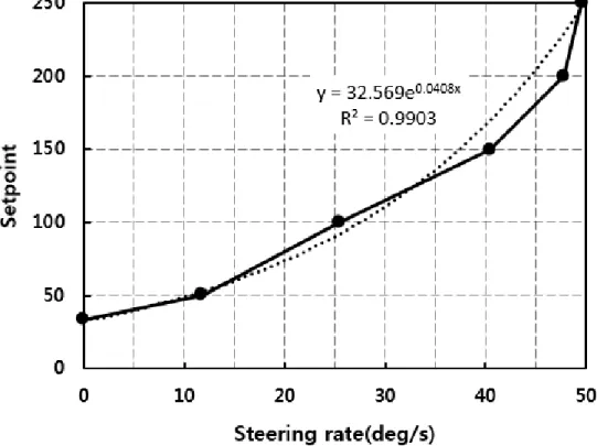
The nonlinear gain function is a valve transform that consists of information regarding the nonlinearity of an E/H valve. Fig. 34 shows the results of the characteristic curves of a steering valve under

various oil flows, i.e., 9.5, 14.5, and 19.3 LPM. Using the HIL

simulator, a valve transform was configured experimentally based on the relationship between the setpoint values of the EHPV and the corresponding steering rates. When the setpoint values are less than 35, the steering cylinder appears to fall into a non-response region. The reasons for the occurrence of a non-response region are mainly due to the influence of the dead band. Comparing the level of performance under three different oil flow conditions, similar

performance curves were obtained at flow rates of 14.5 and 19.3 LPM; however, a large difference was shown at 9.5 LPM. Because the flow conditions of the tractor used in this study are within an

approximate range of about 14.6 to 21.1 LPM, the flow conditions used in the simulator-based experiments were kept constant at 19.3LPM.

The linear model is used as the linear transfer function of the E/H steering system. This model can be mathematically derived from Equation 14 by introducing an inverse nonlinear gain function of the system.

𝐺𝐺𝑙𝑙(𝑠𝑠) = 𝑓𝑓𝑛𝑛−1(𝑢𝑢)𝐺𝐺𝑝𝑝(𝑠𝑠) (14)

Fig. 35 shows the inverse transform of the steering valve. To compensate the dead band of the steering valve, an inverse valve transform model was identified using curve-fitting method.

y = 32.569𝑒𝑒0.0408𝑥𝑥_{, 𝑅𝑅}2 _{= 0.9903 (15)}

The inverse valve transform provides a non-linear control command to quickly actuate the valve spool out of its dead zone.

Fig. 34 Characteristic curves of steering valve at various oil-flow rates obtained experimentally from the HIL simulator.

Fig. 35 Inverse transform of the steering valve, and curve fitting model.

As shown in Equation (16), in fluid dynamics, the volumetric flow rate and the piston speed have a linear relationship.

V =

𝑛𝑛 (16)

where V [𝑐𝑐𝑐𝑐3/s] is the piston speed, Q[𝑐𝑐𝑐𝑐3/s] is the pump

flow rate, and 𝐴𝐴_𝑛𝑛 [𝑐𝑐𝑐𝑐2] is the piston area.

According to the spool characteristic curve, the setpoint and flow rate are linearly related. Therefore, the setpoint and piston speed also have a linear relationship. Based on the maximum steering rate of ±50 deg/s, the output of the P controller was configured to be the input to the inverse transform within the range of -250 to 250. Fig. 36 shows the dead-band compensation model. The dead-band

compensation values of the EHPV for the steering control algorithm are shown in Equation (17).

𝑆𝑆𝑒𝑒𝑆𝑆𝑆𝑆𝑆𝑆𝑠𝑠𝑠𝑠𝑆𝑆𝑑𝑑𝑑𝑑𝑑𝑑𝑑𝑑 𝑏𝑏𝑑𝑑𝑛𝑛𝑑𝑑 = 𝐾𝐾𝑝𝑝𝑠𝑠𝑠𝑠𝑠𝑠(32.569𝑒𝑒0.0082|𝑥𝑥|)(𝜃𝜃𝑑𝑑𝑓𝑓𝑓𝑓𝑓𝑓𝑓𝑓) (17)

Fig. 36 Dead-band compensation model.

2.4.3. Static Friction

There are many sources of friction in such a steering system, including cylinder piston, and the load and side load caused by the road wheels. The friction is highly nonlinear and may adversely affect the performance of the steering control system resulting in steady state errors, limit cycles, and stick-slip motion. Consequently, the road wheels may not follow the steering wheel command as desired. One of the main non-linearities of the cylinder is non-linear friction.

Depending on the application, Coulomb friction and stiction phenomena may have a particularly significant effect on the controller’s performance (Jelali, M., and A. Kroll, 2002). Robotic manipulators must contend with friction which poses a serious challenge to precise manipulator control. Specifically, failing to compensate for friction can lead to tracking errors when velocity reversals are demanded and oscillations when very small motions are required (Leonard. N. E, and P. S. Krishnaprasad, 1992). Coulomb friction is present in hydraulic cylinder seals, although it is only one of the components constituting seal friction characteristics. The basic lubrication mechanism of seals is shown in Fig. 37. It can be seen that the fiction force versus velocity curve is non-linear, particularly at low

cylinder velocities.

Figure 37 Lubrication mechanism of sliding surfaces

To overcome the static friction of a steering cylinder, an impulse-based compensator was proposed in the feedforward loop when the controller received a new steering command for a directional change (Qiu. H. and Q. Zhang, 2003).

In this study, the impulse-based compensator used by Qiu et al. was applied to compensate the static friction of the cylinder. Static friction is the friction that occurs between two or more solid objects

that are not moving relative to each other. In a steering system, static friction appears mainly at the beginning of the change in the direction of the cylinder. Static friction is a problematic in that the controller overreacts by displacing the rod at high speed to compensate for any errors that may occur.

In this study, a simple method is proposed for compensating the static friction that occurs when the direction of the cylinder is

changed. Fig. 38 shows the algorithm used for compensating the static friction during changes in direction. A differentiator of the target angle was used to obtain the direction information of the cylinder. To determine the exact time at which an error occurs from static friction, a threshold value of the steering angle error was set. Impulse mode was activated when the threshold value was exceeded, and during the preset duration (d), a high-magnitude impulse (I) was instantaneously generated to convert the static friction into kinetic friction, as shown in Equation (18). A period of 0.06 s (d) and a magnitude of 80 were found to be sufficient parameters to overcome the static friction in this

study, and where the threshold value(ethres.) was set to 0.2°. The static

friction compensation values to the EHPV for the steering control algorithm are shown in Equation 19.

𝐼𝐼𝑐𝑐𝑆𝑆𝑢𝑢𝐼𝐼𝑠𝑠𝑒𝑒(𝑆𝑆) = �𝐼𝐼, (𝑆𝑆0 ≤ 𝑆𝑆 ≤ 𝑆𝑆0+ 𝑑𝑑) 𝑠𝑠𝑓𝑓 𝜃𝜃𝐷𝐷 ′ _{> 0} −𝐼𝐼, (𝑆𝑆0 ≤ 𝑆𝑆 ≤ 𝑆𝑆0+ 𝑑𝑑) 𝑠𝑠𝑓𝑓 𝜃𝜃𝐷𝐷′ < 0 0, (𝑆𝑆 > 𝑆𝑆0+ 𝑑𝑑) 𝑆𝑆𝑆𝑆ℎ𝑒𝑒𝑒𝑒𝑒𝑒𝑠𝑠𝑠𝑠𝑒𝑒 (18) 𝑆𝑆𝑒𝑒𝑆𝑆𝑆𝑆𝑆𝑆𝑠𝑠𝑠𝑠𝑆𝑆𝑠𝑠𝑡𝑡𝑑𝑑𝑡𝑡𝑡𝑡𝑐𝑐 𝑓𝑓𝑓𝑓𝑡𝑡𝑐𝑐𝑡𝑡𝑡𝑡𝑓𝑓𝑛𝑛= 𝐼𝐼𝑐𝑐𝑆𝑆𝑢𝑢𝐼𝐼𝑠𝑠𝑒𝑒(𝑆𝑆) (19)

where I is the impulse amplitude, d is the impulse duration, and

t0 is the time when the threshold value is exceeded.

Fig. 38 Flow chart of static friction compensator.

2.5. Virtual Terminal

A virtual terminal (VT) is a device for operator interaction with the features of the tractor and agricultural implement. The VT is a control function within an electronic control unit (ECU), consisting of a graphical display and input functions, connected to an ISO 11783 network that provides the capability for a control function, composing an implement or a group of implements to interact with an operator. As shown in Fig. 39, the VT provides the capability to display information and to retrieve data from an operator (ISO 11783-6).

Fig. 39 A VT provides ISO 11783 systems with a graphical display, soft keys, and means to retrieve user inputs

In this study, the VT was constructed to set the auto steering mode as well as to receive the status information of the vehicle in real time. The virtual terminal used a commercial OPUS A3 Eco model

(WACHENDORFF Elektronik, Germany). The VT features 32-bit, 532 MHz processor, with memory 512 MB and two CANBUS ports.

Projektor Tool software is tailored to fit into the ISOBUS development tool chain. Projektor Tool software development suite with graphics development tools and JavaScript capability can be used to reduce programming time. Fig. 40-41 shows screenshot of the Projektor Tool software.

Fig. 40 Screenshot of the Projektor Tool software.

Fig. 41 Screenshot of programming language.

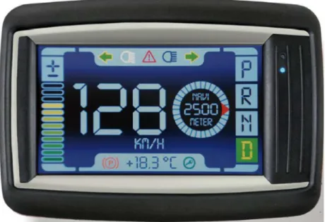
The user interface of the VT consists of main, auto steering status, and positioning status. The main tab is for selecting the other tabs. The auto-steering status tab is shown in Fig. 42. From the auto steering status tab, the user can start or stop the auto steering mode. After the auto steering mode is turned on, the VT sends the message of the guidance system command (PGN 44288). In addition, the VT may real-time receive the vehicle speed, steered wheel angle, and target angle information from CAN bus: Target Angle (0x600), Primary Steered Wheel Angle (0x105), and Speed (PGN 128259).

Fig. 42 The auto steering status tab of the VT contains two functions; activation of the auto steering mode, reading steering information.

The positioning status tab shown in Fig. 43 contains the vehicle heading, vehicle speed, latitude, and longitude information. The VT is configured to receive CAN messages according to the IEC 61162-3 standard: GNSS Position Rapid Update message (PGN 129025), Speed (PGN 128259), and Vessel Heading (PGN 127250).

Fig. 43 The positioning status tab of the VT contains vehicle heading and positioning information