2011 National University of Singapore, Department of Architecture Global Visions: Risks and Opportunities for the Urban Planet
THE LANDSCAPE ECOLOGICAL ASSESSMENT MODEL AND ITS
APPLICATIONS
Dongwoo Lee* & Kyushik Oh**
*Hanyang University, Seoul, Republic of Korea, [email protected] ** Hanyang University, Seoul, Republic of Korea, [email protected]
ABSTRACT: Segregation and fragmentation of the urban ecological landscape can cause a reduction
of biodiversity and result in negative impacts on the atmosphere, energy, water, soil, and ecology. As a result, the quality and functions of the natural landscape can deteriorate, and its aesthetic value can decline. These problems can be resolved by utilizing a landscape ecological approach that minimizes the urban development impacts. This study suggests the landscape ecological assessment model for the stability and bio-diversity of the urban environment. There are four stage of this study: First, important evaluation criteria and standards for landscape ecology were selected. Second, to evaluate landscape ecological performance of an urban area, the landscape ecological assessment model was established. Thirdly, to verify the effectiveness of the model, a case study was conducted using the established assessment model on Byulne City in the Seoul Metropolitan Area. Finally, management policies are suggested to create environment-friendly urban development. The assessment model developed in this study can be used as the basis for analyzing spatial plans and policies and can be viewed as the embodiment of scientific and systematic evaluation through the linking of landscape ecology theory and urban development. It can also contribute toward the preparation of policies regarding environment-friendly planning.
KEYWORDS: Landscape Ecology, Assessment Model, Landscape Ecological Performance, Urban
Development
1 INTRODUCTION
Green space fragmentation due to urban development has reduced the size of various habitats and the amount of biodiversity. The lengthened distance between green spaces have also had a negative impact on the urban ecosystem, interfering with the movements of different animal species. Meanwhile, the perceived importance of landscape ecology quality has been increasing, as seen in the UN announcement of 2010, being the year for ‘bio-diversity.
Therefore, to achieve sustainable urban development, planning tools like ‘Eco-Network’ have been adopted in current urban and environmental conservation planning. However, the problems that have occurred in complex urban spaces commonly contain duplicating and conflicting objectives. Therefore, a systematic assessment tool is necessary to resolve these problems. In this regard, this study developed the landscape ecological assessment model to harmonize conflicting problems in urban spaces. To achieve this, the landscape ecology assessment elements for urban spaces were identified by literature review and assessment methods were established. Next, the landscape ecological assessment model combining urban development and landscape assessment elements was established. To verify the effectiveness of the model, a case study was conducted using the assessment model. The landscape ecological assessment model developed in this study can contribute toward the preparation of policies regarding environment-friendly planning for planning tools of scientific and systematic evaluation.
2 LANDSCAPE ECOLOGICAL ASSESSMENT ELEMENT S
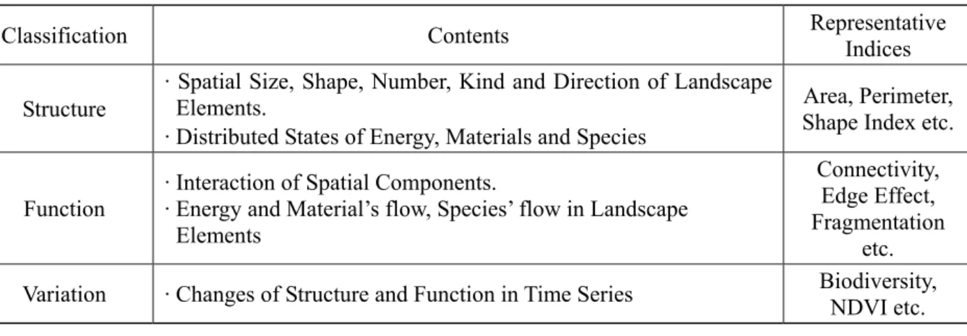
Based on geography and ecology, the notion of landscape ecology created by Neff (1963) and Troll (1968) has been applied to many analyses using remote sensing data. Landscape ecology considers structures on and functions of the landscape, and is useful in resolving ecological problems. In landscape ecology, the landscape is divided into three elements; structure, function and variation.
Landscape structure is the most frequently treated subject in landscape ecology theory research. It determines material flows, animal flows, and energy flows through structure elements. Structure elements like patch size, shape, and corridor characteristics also determine patterns and processes of the landscape (Forman and Godron, 1986). Lee (2001) defined the structure as the spatial relationship of remarkably divided ecological spaces. Thus, structure could be explained by distributed information states which are related to landscape elements like spatial size, shape, number, kind, direction, organization of landscape elements.
Function refers to flows of energy, materials, species, and information which occur through the interaction of landscape elements (Forman and Godron, 1986). In this regard, the structural diversity of landscape ecology is one of the elements for assessing ecological function. Harmonious functions like energy flow, species’ migration, and information movement can be sustained depending on the connectivity strength of a corridor, matrix, and network. The connectivity is the most important for defining ecological structure and dynamics. Most issues for conservation planning essentially require connectivity analysis
Variation refers to changing characteristic or landscape functions in time series. Landscape variation is the most compositive analysis in landscape ecology theory. Research on the relationship of landscape structure and structure elements based on pedology, geography, biology, and the relationship of specific species’ appearance and landscape patterns are major fields of study.
Table 1 Landscape Ecology Assessment Elements
Classification Contents Representative Indices
Structure
· Spatial Size, Shape, Number, Kind and Direction of Landscape Elements.
· Distributed States of Energy, Materials and Species
Area, Perimeter, Shape Index etc.
Function
· Interaction of Spatial Components.
· Energy and Material’s flow, Species’ flow in Landscape Elements
Connectivity, Edge Effect, Fragmentation
etc.
Variation · Changes of Structure and Function in Time Series Biodiversity,
NDVI etc.
3 ESTABLISHMENT OF THE LANDSCAPE ECOLOGICAL ASSESSMENT MODEL 3.1 Assessment Indices
3.1.1 Structure
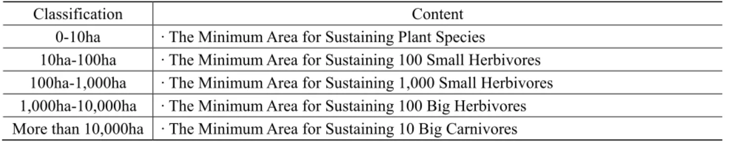
Area, perimeter, and shape index are the most representative indices for analyzing landscape structure. Schonewald-Cox (1983) suggested 10ha as the minimum area for sustaining more than 100 small herbivores. He also suggested 1,000ha for sustaining more than 1,000 small herbivores or more than 100 big herbivores. Weber (2006) also suggested 10ha for an organic green space network. Considering these standards, 2ha was selected for the marginal area.
2
Table 2 Standard for Patch Area
Classification Content
0-10ha · The Minimum Area for Sustaining Plant Species 10ha-100ha · The Minimum Area for Sustaining 100 Small Herbivores 100ha-1,000ha · The Minimum Area for Sustaining 1,000 Small Herbivores 1,000ha-10,000ha · The Minimum Area for Sustaining 100 Big Herbivores More than 10,000ha · The Minimum Area for Sustaining 10 Big Carnivores
Meanwhile, perimeter represents a patch’s winding and roughness, and it has a correlation with biodiversity. Consequently, perimeter is a more important index than area in an invasion context. However, a universal standard cannot be applied because suitable shape is defined by complex components like size, matrix, and other patches. Therefore, shape index has been commonly applied to assessment standard. The shape index is explained by area and perimeter ratio. The low shape index means the patch is similar to a circle, and it causes a positive impact on bio-diversity (Forman and Godron, 1986).
(1) Pi= Perimeter of Patch i
Ai=Area of Patch i
3.1.2 Function
Function assessment refers to evaluating the interaction of patches. To evaluate the functions, fragmentation and connectivity were selected in this study. Fragmentation of patches caused by spatial distribution could be measured using spatial auto-correlation (Turner & Gardener, 1990). Using GIS spatial statistics analysis, specific patches and spatial patterns of the target area could be found. In addition, hot spots (or cold spots) could be delineated. Meanwhile, Moran’s I index can be adopted to measure the spatial autocorrelation, whereby an index near 1 means that similar ones are gathered nearby; 0 means randomly distributed (Moran, P.A.P., 1950). If the Moran’s I index is near -1, it means that the distribution resembles a check pattern. The formula can be presented as follows:
(2)
n= The number of patches indexed by i and j
Xi=The Area (or Shape Index) of Patch i
X= The mean of Xi
Wij= A Matrix of Spatial Weight
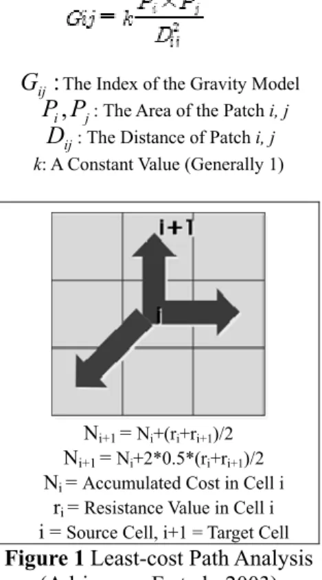
The gravity model is the most basic method for assessing connectivity. Based on physics theory, the gravity model in landscape ecology was found to be very useful to calculate the spatial relationship between each patch. Using the gravity model theory, large areas and short distances were found to cause high connectivity, as opposed to small forest areas and long distances that caused low connectivity (Forman and Godron, 1986). The gravity model theory is shown as equation 3. Meanwhile, Least-cost path analysis is a networking methodology based on landscape permeability theory and raster data set, and is an effective method for constructing ecological networks by considering landscape characteristics. Landscape permeability indicates both the friction value and the geographical position, which are the summed value by reclassification onto a common measurement scale of land cover characteristics, planting type, and slope, etc. The basic structure of the least cost path analysis is shown below (Adriansen. F et al., 2003)
(3)
:
ij
G
The Index of the Gravity Modelj i P
P , : The Area of the Patch i, j
ij
D
: The Distance of Patch i, jk: A Constant Value (Generally 1)
Ni+1 = Ni+(ri+ri+1)/2
Ni+1 = Ni+2*0.5*(ri+ri+1)/2
Ni = Accumulated Cost in Cell i
ri = Resistance Value in Cell i
i = Source Cell, i+1 = Target Cell
Figure 1Least-cost Path Analysis (Adriansen. F et al., 2003)
3.1.3 Variation
The most common method to assess variation is biodiversity. Biodiversity is the degree of variation of life forms within a given ecosystem, biome, or an entire planet. Thus, it means measuring the health of ecosystems. The location of habitats of varieties could be applied to variation assessment. NDVI (Normalized Difference Vegetation Index) was applied to identify the variation of the path’s vitality. NDVI can be calculated by landsat remote sensing data. However variation index was not considered in this study due to a lack of time series data.
(4)
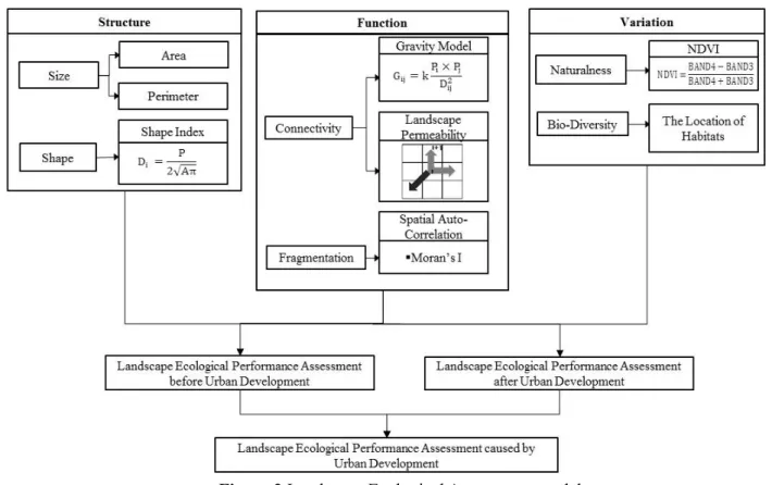
3.2 The Landscape Ecological Assessment Model
The landscape ecology assessment model measures variation of landscape ecological performance caused by urban development projects. The landscape ecology performance of a development area can be assessed by a combination of structure, function, and variation. For example, green space conservation assessment could be conducted by analysis of structure index such as area, perimeter, and shape index. Next, a landscape ecological function like fragmentation could also be measured using spatial auto-correlation analysis. The connectivity assessments for enhancing the landscape function could be conducted using the gravity model and landscape permeability analysis. The ecologially deterioration area could also be found using variation assessment like NDVI and biodiversity. Based on these assessment characteristics, the previous ecological state and subsequent state were compared (Figure 2).
2
Figure 2 Landscape Ecological Assessment model 4 CASE STUDY
4.1 The Study Area
The study area is the ‘Byulne’ urban development project of the capital region, i.e. the Seoul Metropolitan Area. This area had been removed from the green belt area by national policies and subsequently, large urban development projects were planned. The development area is about 5km2 and 76,000 people will inhabit this area.
4.2 Results
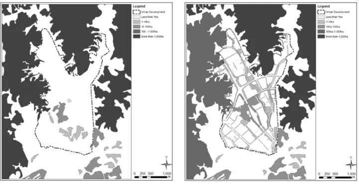
4.2.1 Structure (Size, Shape)
The number of patches has increased from 8 to 196 after urban development. As a result, the total patch area has also increased form 43.72ha to 97.96ha. However, the average area has decreased about 4.8ha (Figure 4). This result was caused by variously planned patch types like parks, corridors, and buffers. Meanwhile, the number of patches that meet the minimum area for sustaining plant species (2ha) were 10. Consequently, the structural performance has improved in terms of scale. However, the average shape index has increased from 0.008 to 0.032. This means that the patch shape changed from a circle shape to an angular shape, and it also means that the patch shapes changed negatively in terms of bio-diversity (Figure 5).
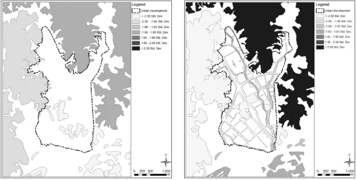
4.2.2 Function (Fragmentation)
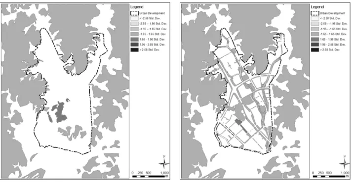
The patch fragmentation patterns based on area were determined as cold spots (Z<2.58) in all states (before and after the development state). As regional Moran’s I changed from 0.1 to 0.03, the fragmentation increased a little after development. This means fragmentation of small patches occurred in the study area (Figure 6). These results were caused by the location of large patches near the study area. The large patch of the northern area changed into a hot spot as the number of small patches sharply increased after development. The patch fragmentation patterns based on shape index was determined randomly in all cases, and a little clustering was found to have occurred after development (Figure 7). Meanwhile, the average distance of patches decreased from 2,445m to 1,569m. Consequently, the fragmentation condition was improved after urban development, considering increases of the number and size of the patches.
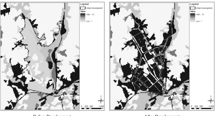
4.2.3 Function (Connectivity)
The connectivity assessment result based on the gravity model showed the number of patches networks increased about fourfold (Figure 8). However, a sixfold decrease of the gravity index occurred after development. This result was caused by an individually insufficient patch area securement compared with the number of patch increase. This also means that a large patch area could not be secured due to a road network plan. Meanwhile, the connectivity assessment result based on landscape permeability showed the friction value increased by eighteenfold. This was the result of landcover, like flora, which is suitable for animal migration, being changed into urban areas after development (Figure 9).
G Before Development
G After Development
2
Before Development After Development
Figure 5 Structure (Shape)
Before Development After Development
Before Development After Development Figure 7 Fragmentation (Shape)
Before Development After Development
Figure 8 Connectivity (Gravity Model)
2
Before Development After Development
Figure 9 Connectivity (Landscape Permeability)
4.2.4 The Landscape Ecological Variation Caused by Urban Development
Urban development has resulted in positive effects like patch number increase, total area increase, and fragmentation improvement in the study area. However, the negative impacts such as average shape index increase and connectivity decline also occurred (Table 3). Negative impacts were caused by landcover variations and road network construction. These negative impacts disturbed sufficient patch area securement for meeting landscape ecological functions. Therefore, once the fragment areas are connected through the establishment of an underground road, eco-bridge etc., a sufficient area will be secured and connectivity will be enhanced to improve landscape ecological performance in the study area.
Table 3 Comparison of Landscape Ecological Performance (Before development vs After development)
Classification Development Before Development After Result
Structure
The Number of Patches 8 196 Improved
Area Total Area (ha) 43.72 97.96 Improved
Average Area (ha) 5.46 0.62 Declined
Average Shape Index 0.008 0.032 Declined
Fragmentation
Average Distance (m) 2,445 1,569 Improved
Area (Moran's I) 0.1 (Clustered) 0.03 (Clustered) Declined
Shape Index (Moran' I) -0.04 (Random) -0.01 (Random) Improved
Connectivity Gravity model The Number of Networks 18 70 Improved Average Gravity Index 12,013 2,227 Declined
5 CONCULUSION
This study developed the landscape ecological assessment model and suggested its applications. The assessment model was established in consideration to ecological issues such as structure, function, and variations in urban space. The measurable and concrete results based on landscape ecology were deducted using this model. The improved elements and declined elements caused by urban development were also determined using this model. However, the variation indices of landscape ecology were not considered due to a lack of time series data in this study. Moreover, regional impacts such as cumulative impacts caused by urban development were not considered. Nevertheless, this study suggests the landscape ecological assessment model for concrete results. The established model in this study can be utilized as an effective decision-making tool for urban environmental management and to enhance biodiversity in urban areas.
ACKNOWLEDGEMENT
This work was supported by a Korea Science and Engineering Foundation (KOSEF) grant provided by the Korean Ministry of Education, Science and Technology (MEST) (No. R01-2008-000-20348-0)
REFERENCES
[1] Moran, P.A.P., “Notes on Continuous Stochastic Phenomena,” Biometrika, Vol. 37 (1950), pp.17-33 [2] Schonewald-Cox, C.M., “Guidelines to management: A beginning attempt,” Sunderland,
Messachusetts: Sinauer Associates, Inc., 1983.
[3] Forman, R.T.T., and M. Godron, “Landscape Ecology,” New York, USA, John wiley & Sons, Inc., 1986.
[4] Forman, R.T.T., “Land Mosaics: The Ecology of Landscape and Regions,” Cambridge University Press, New York, Inc., 1995.
[5] Turner, M.G., R.H. Gardner, and R.V. O'nell, “Landscape Ecology in Theory and Practice,” Springer Science Business Media, Inc., 2001.
[6] Lee, D.W., “Landscape Ecology Theory,” Seoul National University Press, 2001.
[7] Cook, E.A., “Landscape Structure Indices for Assessing Urban Ecological Networks,” Landscape and Urban Planning, Vol.58 (2002), pp.269-280.
[8] Adriaensen, F. et al., “The Application of Least-cost Modeling as a Functional Landscape Model,” Landscape and Urban Planning, Vol.64 (2003), pp.233-247.
[9] Weber, T., A. Sloan, and J. Wolf, “Maryland’s Green Infrastructure Assessment: Development of a Comprehensive Approach to Land Conservation,” Landscape and Urban Planning, Vol. 58 (2006), pp.157-170