1. INTRODUCTION
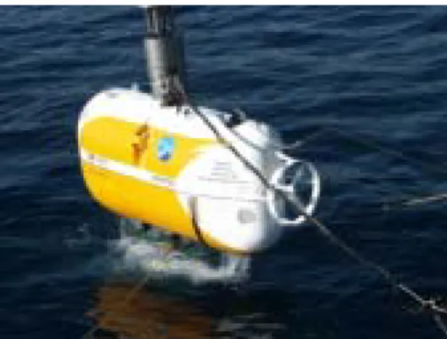
Fig.1 Autonomous Underwater Vehicle ‘MR-X1’
Although 70 percents on the surface of the Earth is the ocean, a lot of unexplored parts have been left. In these days, efficient investigations of the ocean and the seabed have been interested. However, undersea is the extreme environment that we can’t step into easily. Therefore operating robots for taking over from human being is desired. If such kind of robots had been developed, we can avoid danger.
In order to realize it, an Independent Administrative Corporation Japan Agency for Marine-Earth Science and Technology (JAMSTEC) is developing light-and-small Autonomous Underwater Vehicles (AUV) to explore the ocean. The AUV named ‘MR-X1’ (Marine Robot Experimental 1) can cruise, investigate and observe by itself without human’s help. In order to be able to turn in a small space and explore efficiently, ‘MR-X1’ has five thrusters. One main thruster is for the forward and the backward motion, two thrusters are for the horizontal motion and two thrusters are for the vertical motion.
In this paper, the motion control problem of this AUV ‘MR-X1’ is considered. In order to operate ‘MR-X1’, five thrusters have to be controlled appropriately. Since two vertical thrusters set up by inclining from the perpendicular, if these vertical thrusters are rotated, ‘MR-X1’ not only moves the vertical direction but also moves the horizontal direction. In the case of considering the cruising ‘MR-X1’ with the constant altitude, both vertical and horizontal thrusters have to be controlled appropriately. The present paper considers that ‘MR-X1’ is controlled to make it go straight on surge direction, and stop at the targeting point with the constant altitude.
Since the dynamic property of ‘MR-X1’ is changed by the influence of the speed, the mathematical model of ‘MR-X1’ becomes the nonlinear model. In order to design a controller for ‘MR-X1’, we generally apply nonlinear control theories or linear control theories with some constant speed situation. If the controller is designed by applying the Linear Quadratic
(LQ) optimal control theory, the obtained controller only compensates the optimality at the designed speed situation, and does not compensate the stability at another speed situations. In order to solve this problem, this paper proposes a controller design method using Linear Matrix Inequalities (LMIs), which can adapt the speed variation of ‘MR-X1’. By applying this method, we will be able to find suitable gain on the speed variation of ‘MR-X1’. And examples of numerical analysis using our designed controller are shown.
The design method research of the control system for Autonomous
Underwater Vehicle (AUV) using Linear Matrix Inequality (LMI)
Youhei Nasuno
*, Etsuro Shimizu
**,
Taro Aoki
***, Ikuo Yomamoto
***, Tadahiro Hyakudome
***,
Satoshi Tsukioka
***, Hiroshi Yoshida
***, Shojiro Ishibashi
***,
Masanori Ito
**, Ryoko Sasamoto
****,
* Department of Marine System Engineering, Tokyo University of Marine Science and Technology, Tokyo, Japan (Tel: +81-5245-7300; E-mail: [email protected])
**Department of Marine Mechanical Engineering, Tokyo University of Marine Science and Technology, Tokyo, Japan ***Marine Technology Center, Japan Agency for Marine-Earth Science and Technology (JAMSTEC), Kanagawa, Japan
****Department of Electrical Mechanical Engineering, Tokyo University of Marine Science and Technology, Tokyo, Japan Abstract: An Independent Administrative Corporation Japan Agency for Marine-Earth Science and Technology (JAMSTEC) is
developing light-and-small Autonomous Underwater Vehicles (AUV)1)
, named ‘MR-X1’ (Marine Robot Experimental 1), which can cruise, investigate and observe by itself without human’s help. In this paper, we consider the motion control problem of ‘MR-X1’ and derive a controller. Since the dynamic property of ‘MR-X1’ is changed by the influence of the speed, the mathematical model of ‘MR-X1’ becomes the nonlinear model. In order to design a controller for ‘MR-X1’, we generally apply nonlinear control theories or linear control theories with some constant speed situation. If we design a controller by applying Linear Quadratic (LQ) optimal control theory, the obtained controller only compensates the optimality at the designed speed situation, and does not compensate the stability at another speed situations. This paper proposes a controller design method using Linear Matrix Inequalities (LMIs)2),3),4), which can adapt the speed variation
of ‘MR-X1’. And examples of numerical analysis using our designed controller are shown.
Keywords: Autonomous Underwater Vehicle (AUV), MR-X1 (Marine Robot Experimental 1), Linear Quadratic (LQ) optimal control, Linear Matrix Inequality (LMI), Equation of motion
Table 1 Principal specification of ‘MR-X1’
Dimensions 2.5[m](total length) × 0.8[m](width) × 1.2[m](height) Weight 800[kg] (in the air)
Cruising Speed 2[kt]
Maximum Depth 4200[m]
Actuators 1. Main thruster (400W)
2. Two horizontal thrusters (150W) 3. Two vertical thrusters (150W)
2. EQUATION OF MOTION FOR ‘MR-X1’
M :Inertial MatrixC(ν) :Matrix of Coriolis and Centripetal Terms 2.1 Coordinate system
) :Damping Matrix D(ν
In this paper, we use two coordinate systems. One is the Earth-fixed coordinate system and the other is the Body-fixed coordinate system. Fig.2 shows the relation between each coordinate system. In general, linear and angular velocities are represented by using Body-fixed coordinate system, but the translation to the Earth-fixed coordinate system is suitable to observe the motion of ‘MR-X1’. The matrix of coordinate transformation between the Earth-fixed coordinate system and the Body-fixed coordinate system becomes as follow.
g(η) :Matrix of Restoring Forces and Moments τ :Thrusts
2.2.1 Inertial Matrix
Inertial matrix is defined as the sum of inertial mass matrix and added inertial matrix due to the inertia of the urrounding fluid. RB M MA s A RB M M M≡ + (2.4) 0 X 0 Y Z0 X1 -MR O X Y Z (surge) u (heave) w (sway) v (pitch) q (yaw) r (roll) p 0 r system coordinate fixed -Body system coordinate fixed Earth − − − − = zz G xx G G G yy G G G G RB I mx I mz mx mz m I mx mz mx m mz m M 0 0 0 0 0 0 0 0 0 0 0 0 0 0 0 0 0 0 0 0 0 0 (2.5) − ≡ 66 44 22 55 33 11 0 0 0 0 0 0 0 0 0 0 0 0 0 0 0 0 0 0 0 0 0 0 0 0 0 0 0 0 0 0 A A A A A A MA (2.6)
Position of the center of gravity of ‘MR-X1’ can be represented as [ ] with the Body-fixed coordinate system. It is assumed that the product of inertia is 0, because ‘MR-X1’ has the symmetrical configuration. Furthermore, the added mass is also 0 except diagonal elements. G G z x ,0, T ∗ ∗ I ∗ ∗ A
Fig.2 Coordinate system of ‘MR-X1’
ν η
η•=J( ) (2.1)
T :Position and angle vector with
the Earth-fixed coordinate system y
z
x, , , , , ] [ ϑ φ ϕ η=
T :Linear and angular velocity vector
with the Body-fixed coordinate system r p v q w u, , , , , ] [ = ν
2.2.2 Matrix of Coriolis and Centripetal Terms
The matrix of coriolis and centripetal terms is defined as the sum of the coriolis matrix of Rigid-body CRB(
ν
) and thecoriolis matrix in ideal fluid CA(
ν
).:Position z y x ,, ϕ ϑ φ, , :Angle :Linear velocity w v u ,, :Angular velocity r q p ,, (ν) (ν) (ν) (2.7) A RB C C C ≡ + + − − + = ϑ φ ϑ φ φ ϕ ϑ φ ϕ ϑ ϕ φ φ ϑ ϑ ϑ φ ϕ φ ϕ ϑ ϕ η cos / sin 0 0 tan sin 0 0 0 cos sin sin sin cos cos sin cos 0 0 0 cos cos sin 0 sin cos cos sin sin cos cos ) ( J − − + − − + + − + − − − = p I p mx v r x m r I v p z m r mz p x r z m u q z m w q x m u q z m w q x m C xx G G zz G G G G G G G G RB ) ( ) ( ) ( 0 0 0 ) ( ) ( ) ( 0 0 ) ( 0 0 + − + − ϑ φ ϑ φ ϕ ϑ φ φ ϕ φ φ ϑ φ ϑ ϕ φ ϕ cos / cos 0 0 tan cos 1 0 0 0 sin sin sin cos cos sin 0 0 0 0 sin cos 0 0 sin sin cos cos sin − − − − + − + − − + − 0 0 0 ) ( ) ( ) ( 0 ) ( 0 q I mu q I mw mu mw p I r I p x r z m q y p x m v p z m v r x m r mz yy yy xx zz G G G G G G G (2.2) (2.8)
) :Velocity transformation matrix (η J − − − − − − − − − = 0 0 0 0 0 0 0 0 0 0 0 0 0 0 0 0 0 0 55 11 44 22 55 33 66 22 11 33 44 66 11 33 22 11 22 33 q A u A p A v A q A w A r A v A u A w A p A r A u A w A v A u A v A w A CA 2.2 Dynamics of ‘MR-X1’
The motion of underwater vehicle is represented as the 6DOF nonlinear equation5). In general, its motion can be
treated as the motion of Rigid-body. The nonlinear equation is epresented as (2.9) r τ η ν ν ν ν ν•+C( ) +D( ) +g( )= M (2.3)
where 2.2.3 Damping Matrix
The damping matrix of ‘MR-X1’ in the fluid is represented
s XTHM nTHMnTHM DTHM KT 4 ρ = 01724 . 0 84628 . 0 n Y = + (2.13) a 2 3 0155 . 0 THF THF THF THF n + n 3 2 (2.14) } , , , , , { ) ( diag Xu Zw MqYv Kp Nr Dν =− 0.98582 0.02722 0.01577 THR THR THR THR n n n Y = + + 3 2 (2.15) } , , , , , {X||u Z | |w M||q Y||v K || p N||r diag uu ww qq vv pp rr − 0.95576 0.02028 0.01512 TVL TVL TVL TVL n n n Z = + + 3 2 (2.16) 01526 . 0 02204 . 0 96669 . 0 TVR TVR TVR TVR n n n Z = + + (2.17) − = r v r v r v q w q w N N K K Y Y M M Z Z 0 0 0 0 0 0 0 0 0 0 0 0 0 0 0 0 0 0 0 0 0 0 0 0 0 0 THM n THF n THR n
:Rotational speed of the main thruster
:Rotational speed of the front horizontal thruster
TVL
n
TVR
n
:Rotational speed of the rear horizontal thruster :Rotational speed of the portside vertical thruster :Rotational speed of the starboard vertical thruster
+ + + + − r N r N v N p K r Y r Y v Y q M q M w M q Z q Z w Z v X w X u X rr vr vv pp rr vr vv qq wq ww qq wq ww vv ww uu 0 0 0 0 0 0 0 0 0 0 0 0 0 0 0 0 0 0 0 0 0 0 0 0 α 48 . 0 = THM D
The first term is the force and the moment of the first order of the velocity, and the second term is the second order of the velocity. These values of the matrix components are obtained from experiments.
2.2.4 Restoring Forces and Moments
The position of the force of buoyancy of ‘MR-X1’ can be represented as [ ]T with the Body-fixed coordinate
ystem, so the restoring forces and moments are represented as
B B z x,0, s − − − − − − + − − − − = φ θ φ θ φ θ φ θ θ φ θ θ η sin cos ) ( sin cos ) ( sin cos ) ( cos cos ) ( sin ) ( cos cos ) ( sin ) ( ) ( B x W x B z W z B W B x W x B z W z B W B W g B G B G B G B G where
W:Force of gravity, B:Force of buoyancy 2.2.5 Thrusts
In this paper, the following expression is used as the mathematical model of thrusts of ‘MR-X1’. These components are the function of the rotational speed of
hrusters. t ⋅ − ⋅ + ⋅ + ⋅ − ⋅ + ⋅ + ⋅ − ⋅ − ⋅ + ⋅ − + − − − ⋅ + ⋅ + ⋅ − + = α α α α α αα α α α α α τ sin sin cos sin cos sin sin sin cos cos cos cos TVR TVR TVL TVL THR THR THF THF TVR TVR TVR TVR TVL TVL TVL TVL THR THR THF THF TVR TVL THR THF TVR TVR TVL TVL THM THM TVR TVL THM Z x Z x Y x Y x Z y Z z Z y Z z Y z Y z Z Z Y Y Z x Z x X z Z Z X THM X THF Y THR Y TVL Z TVR Z ] , , [xTHF yTHF zTHF ] , , [xTHR yTHR zTHR ] , , [xTVLyTVLzTVL ] , , [xTVRyTVRzTVR 171 . 0 = T K = ρ 1025
:Declination of vertical thrusters [rad] :Diameter of the main thruster [m] :Thrust coefficient
:Fluid density [kg/m3]
(2.10)
These thrusters have following limitations.
5 5≤ ≤
− nTHM
,
−12≤nTHF,nTHR,nTVL,nTVR≤123. D
ESIGNING A CONTROL SYSTEM FOR‘MR-X1’
The aim of developing ‘MR-X1’ is to construct the autonomous underwater vehicle that it not only follows the given path but also stops at the objective point and keeps the point to investigate, observe and operate. In order to realize these, five thrusters equipped on ‘MR-X1’ have to be controlled to be appropriate rotational speeds. In order to know the dynamic characteristic of ‘MR-X1’, the main thruster was only rotated firstly. Since the displacement toward to the heave direction occurred, to keep constant altitude, two vertical thrusters have to be rotated. However, vertical thrusters set up by heaving the inclination from the perpendicular. If these thrusters are rotated, ‘MR-X1’ not only moves the vertical direction but also changes the horizontal direction. Therefore, in the case of cruising ‘MR-X1’ with the constant altitude, these five thrusters have to be controlled appropriately. The present paper considers the controller design problem for ‘MR-X1’ to make it go straight on surge direction, and stop at the objective point with the constant altitude. It is obvious that this mechanical model of ‘MR-X1’ depends on the speed of each direction; surge, sway and heave. In order to design a controller, we have to consider effects of these speed variations. However, in our problem, the main thruster is used the different way compared with other thrusters; the main thruster is used for the straight cruising toward the surge direction with speed u, and other thrusters are used for holding attitude or following the path. This means that if other thrusters are controlled appropriately from the start, variations of speeds for vertical and horizontal directions can be controlled to become variation sufficiently small and we need not to consider effects of variations of speeds. Therefore, in this paper, we design a control system to adopt the variation of the speed for the surge direction.
(2.11)
(2.12)
:Thrust of the main thruster
:Thrust of the front horizontal thruster :Thrust of the rear horizontal thruster :Thrust of the portside vertical thruster
3.1 Linearization :Thrust of the starboard vertical thruster
In order to design a control system, we divide the mechanical model ‘MR-X1’ into surge motion part and the others and linearize the other part of the mechanical model except the surge direction speed u. The speed u is used as a parameter. Furthermore, the pitch angle and the pitch rate are :Position of the front horizontal thruster
:Position of the rear horizontal thruster :Position of the portside vertical thruster :Position of the starboard vertical thruster
neglected, because the control of the pitch angle is difficult from the constitutional character of ‘MR-X1’. The linearized
odel is shown as follows.
3.3 Designing a control system
In this section, the control system is designed to control ‘MR-X1’ moving toward the objective point. The control system is firstly designed using the linear quadratic (LQ) optimal control. Generally, in order to design the LQ optimal control system for linear systems, it is necessary to solve the Algebraic Riccati equation by using constant matrices A and B in the state equation. Since the Riccati equation is solved easily by using some computer softwares, the state feedback control system can be easily obtained. In order to apply the LQ control theory for ‘MR-X1’, we have to fix the cruising speed u. Therefore, the optimality of the obtained control system is only compensated about the one speed. However, the obtained control system does not compensate the stability in other speed situations.
m
⃝Matrix of coordinate transformation
= 1 0 0 0 0 1 0 0 0 0 1 0 0 0 0 1 ) (η J (3.1) ⃝Inertial matrix − − − − − − = 66 44 22 33 0 0 0 0 0 0 0 0 A I mx A I mz mx mz A m A m M zz G xx G G G L (3.2)
⃝Matrix of coriolis and centripetal terms In order to compensate the stability, we propose the new design method by using the LMI, which correspond to the Riccati inequality. The algorithm to solve the LMI has a property that can solve some number of LMIs simultaneously. By applying this property, it is considered that we can obtain the solution that satisfies the LMI condition under several speeds. The proposed strategy to design the control system is represented as follow. − − − = 0 0 ) ( 0 0 0 0 0 ) ( 0 0 0 0 0 0 0 ) ( 11 11 u A m u A m CLν (3.3) ⃝Damping matrix − = r v r v r v w L N N K K Y Y Z D 0 0 0 0 0 0 0 0 0 )
(ν (3.4) optimal control on state equation (3.8) is represented as The LMI that corresponds to Riccati equation in LQ 0 ) ( ) ( < − − + I CX XC BB u XA X u A T T T i i (i=0,…,m) (3.11)
⃝Matrix of restoring forces and moments
− = 0 0 0 0 0 0 0 0 0 0 0 0 0 0 0 ) ( B z W z g B G L Lη 0 > X (3.5)
The constant matrix C corresponds to the weighting matrix in LQ optimal control. The speed parameter u including LMI is given appropriately. By applying the algorithm to solve the LMIs, we can obtain one solution X. In this case, the control
nput τ is represented as ⃝State variable T L L, ] [η ν = (3.6) x i where τ =−BTX−1x (3.12) ] , , , [ZYφϕ L= νL=[w,v,p,r]
η , Note that the solution X satisfies LMI conditions on all
speed parameters. This means that the obtained control system compensates the stability for all speed situations, which substitute for parameters u.
⃝Thrusts • − − + − − − − − − = α α α α α α α α α α τ sin sin cos sin cos sin sin sin 1 1 cos cos 0 0 TVR TVL THR THF TVR TVR TVL TVL THR THF L x x x x y z y z z z
4. SIMULATIONS
96669 . 0 0 0 0 0 95576 . 0 0 0 0 0 98582 . 0 0 0 0 0 84628 . 0 4.1 Simulation conditions (3.7)Table 2 Requirements of simulations
Simulation time 600[sec] Initial position [-30.0(m), 1.0(m), 1.0(m)]
Target point [0(m), 0(m), 0(m)] 3.2 State Equation
The state equation of ‘MR-X1’ is represented as τ B x u A x= + • ) ( (3.8)
For LQ optimal control systems, two types of simulations were done. One is the optimal gain for the surge speed 0[m/s] (Case 1), and the other is for 0.3[m/s] (Case 2). The speed of 0[m/s] corresponds to keeping the objective point. The speed 0.3[m/s] is the middle speed of ‘MR-X1’ since the maximum speed of ‘MR-X1’ is about 0.6[m/s]. On the other hand, for LMIs, we simulated using the controller that derived by substituting speed parameters between 0[m/s] and 0.7[m/s] (Case 3). T T L L ZY wv pr x=[η ,ν ] =[ , ,φ,ϕ, , , , ] • • • • • • • • • • • :State variable T T L L ZY wv pr x=[η ,ν ] =[ , ,φ,ϕ, , , , ] T TVR TVL THR THF n n n n , , , ] [ = τ :Input − + − = × − − 4 4 1 1 0 ) ( ) ( } ) ( { L L L L L L L L J g M D u C M A η η (3.9) = × − 4 4 1 0 τ L M B (3.10)
4.2 Simulation results ⃝Case 1
Starting point
Ending point
Fig.6 Displacement of ‘MR-X1’ in3−D visualization
The ‘MR-X1’ does not always cruise with the constant speed. Therefore, when speed changing occurs, the optimal gain will fluctuate in each case, and if we use the control system that derived under one fixed speed like this simulation, the obtained control system cannot compensate the stability at other speed situations, ‘MR-X1’ tends to diverge like Fig.5 and Fig.6.
Fig.3 Variation in linear velocity with transition of the time
⃝Case 3
Starting point Ending point
Fig.4 Displacement of ‘MR-X1’ in3−D visualization
The movement from the initial position to the objective point occurs the velocity consequently, so the control system of 0[m/s] cannot compensate the stability at the speed occurring, and ‘MR-X1’ tends to diverge like Fig.3 and Fig.4.
Fig.7 Variation in linear velocity with transition of the time
⃝Case 2
Starting point
Ending point
Fig.8 Displacement of ‘MR-X1’ in3−D visualization Fig.5 Variation in linear velocity with transition of the time
Initial deflections of Y-axis and Z-axis converge to the desired path on X-axis. The speed of ‘MR-X1’ is reduced and becomes 0[m/s] at the origin.
5. CONCLUSIONS
In this paper, the mathematical model of Autonomous Underwater Vehicle named ‘MR-X1’, which is developing at JAMSTEC, was derived. We set the aim on autonomous tracking given path and stopping at the objective point, and for this aim, we applied LQ optimal control system and LMIs. In the result, LMIs made it possible to design a control system that corresponds to speed changing, and showed the robustness. It has more effective performance than LQ optimal control system.
Now, this development is in the stage of performance test. We are going to confirm this simulation results with sea-trial of ‘MR-X1’.
REFERENCES
[1] Hiroshi Yoshida: A Working AUV for Scientific Research, OCEAN ’04 MTS/IEEE, TECHNO-OCEAN ’04, Nov.9-12, 2004, Kobe, Japan
[2] P.Apkarian, G.Becker, P. Gahinet, H.Kajiwara: LMI Techniques in Control Engineering from Theory to Practice, IEEE CDC ’96 Workshop, 1996
[3] Ikuo Yamamoto: Marine Control System, International Journal of Robust and Nonlinear Control, Vol.11, No.13, 2001
[4] Tetsuya Iwasaki: LMI and Control, Shokodo, 1997 [5] Thor I.Fossen: Guidance and Control of Ocean Vehicles,