ICCAS2005 June 2-5, KINTEX, Gyeonggi-Do, Korea
Hybrid Controller of Neural Network and Linear Regulator for Multi-trailer Systems
Optimized by Genetic Algorithms
MUHANDO Endusa†, KINJO Hiroshi∗, UEZATO Eiho∗ and YAMAMOTO Tetsuhiko∗
†Graduate School of Engineering & Science, Mechanics and Control Engineering, University of the Ryukyus, 903-0213 JAPAN
(Tel: +81-80-1723-1351; Email: [email protected])
∗Mechanical Systems Engineering, University of the Ryukyus, Senbaru 1, Nishihara, Okinawa, 903-0213 JAPAN
(Tel+Fax: +81-98-895-8632; Email: (kinjo,uezato,yamamoto)@tec.u-ryukyu.ac.jp)
Abstract: A hybrid control scheme is proposed for the stabilization of backward movement along simple paths for a vehicle composed of a truck and six trailers. The hybrid comprises the combination of a linear quadratic regulator (LQR) and a neurocontroller (NC) that is trained by a genetic algorithm (GA). Acting singly, either the NC or the LQR are unable to perform satisfactorily over the entire range of the operation required, but the proposed hybrid is shown to be capable of providing good overall system performance. The evaluation function of the NC in the hybrid design has been modified from the conventional type to incorporate both the squared errors and the running steps errors. The reverse movement of the trailer-truck system can be modeled as an unstable nonlinear system, with the control problem focusing on the steering angle. Achieving good backward movement is difficult because of the restraints of physical angular limitations. Due to these constraints the system is impossible to globally stabilize with standard smooth control techniques, since some initial states necessarily lead to jack-knife locks. This paper demonstrates that a hybrid of neural networks and LQR can be used effectively for the control of nonlinear dynamical systems. Results from simulated trials are reported.
Keywords: Hybrid controller, LQR, Neurocontroller, Genetic algorithm, Trailer backward movement control.
1. Introduction
The control problem for the trailer truck system is known to be one of the highly non-linear, multi-variable and un-stable control problems. Difficult in control intensifies with increase in the number of trailers. The system presents sat-urations on the steering angle and on the relative angles be-tween the trailers. These constraints present a challenging problem of unstable nonlinear dynamics. The control task is to back up the vehicle to a desired trajectory without getting out of control and without expriencing jack-knife locks.
Soft computing techniques, notably Fuzzy technology and Neural computing have found major applications in engi-neering design and manufacturing [1]. Unlike fuzzy methods that use ’vague’ data sets, neural networks are well adapted to nonlinear systems due to their ability to learn [2]. They are well suited for the trailer backward control problem as learning is enhanced by the availability of quantifiable train-ing data. Further, suitable genetic algorithms (GAs) can be modeled to offer a powerful training base [3].
Many control systems for the problem have been pro-posed. Earlier works by Tanaka et al. [4,5] have shown that fuzzy control exhibits good control performance. With regard to the neurocontrol system, Nguyen and Widrow [6] reported the pioneering work for the neurocontrol applica-tion on the trailer-truck system. They successfully designed a controller utilizing a back-propagation (BP) algorithm. Jenkins and Yuhas [7] have presented a small-sized neuro-controller (NC), also based on BP. In previous studies, Kinjo et al. proposed various control methods for a single trailer-truck combination, for a trailer-truck connected to two trailers and for a five trailer-truck combination, using NCs evolved by GA [8-10]. Though evolution of the NCs for the designs were successful, the methods are computationally expensive.
In this study, we present the concept of a hybrid con-trol system comprising the linear quadratic regulator (LQR) for the linear part and the NC for the nonlinear part. Our main motivation derives from the fact that the aforemen-tioned methods fall short of globally stabilizing the control object. The LQR alone can not offer the full control per-formance due to the nonlinear characteristics of the control object. Likewise, the NC on its own is not very efficient as the method takes many training times to evolve the NCs and sometimes the evolution fails. To tackle these problems our proposed hybrid utilizes a synthesis of both control outputs of the LQR and NC. Our prime focus is twofold: to control the steering angle such that the system does not yield the out of control states, and minimizing the physical limitations of the angular differences thereby avoiding the jack-knife phe-nomenon.
The remainder of this paper is organized as follows. The model of the trailer-truck system is presented in Section 2. Section 3 explains the hybrid concept that incorporates the LQR and NCs. Simulation results are shown in Section 4 while a discussion on performance of the scheme follows in Section 5. We draw some general conclusions and our per-spectives in Section 6.
2. Modeling and Problem Formulation
2.1. The Trailer-truck Model
Figure 1 details the geometry of our control object: the six trailer-truck model with an actuated front steering, and its orientation in a coordinate base. Table 1 explains the ter-minology used for the trailer-truck system parameters. The steering angle u(t), is the input to the system and is deter-mined by the state variables x1− x13. The kinematics of the
system are described by the set of equations (1) - (15).
0 L L L l L L L x5(t) x1(t) x2(t) x3(t) x4(t) x6(t) x7(t) x8(t) x9(t) x10(t) x11(t) x12(t) x13(t) x14(t) u(t) x0(t)
Fig. 1. Schematic model of the trailer-truck Table 1. Parameters of the trailer-truck system
Quantity Description
l Truck length
L Trailer length
∆t Sampling time
v Speed of system
u(t) Steering angle
x0, x2, x4, x6, Angles of truck, 1st, 2nd, 3rd,
x8, x10and x12 4th, 5th and 6th trailers
Angular Differences, between: x1 Truck and 1st trailer
x3 1st and 2nd trailer
x5 2nd and 3rd trailer
x7 3rd and 4th trailer
x9 4th and 5th trailer
x11 5th and 6th trailer
x13 Vertical position of 6th trailer
x14 Horizontal position of 6th trailer
x0(t + 1) = x0+v∆tl tan[u(t)] . . . (1) x1(t) = x0(t) − x2(t) . . . (2) x2(t + 1) = x2(t) +v∆tL sin[x1(t)] . . . (3) x3(t) = x2(t) − x4(t) . . . (4) x4(t + 1) = x4(t) +v∆tL sin[x3(t)] . . . (5) x5(t) = x4(t) − x6(t) . . . (6) x6(t + 1) = x6(t) +v∆tL sin[x5(t)] . . . (7) x7(t) = x6(t) − x8(t) . . . (8) x8(t + 1) = x8(t) +v∆tL sin[x7(t)] . . . (9) x9(t) = x8(t) − x10(t) . . . (10) x10(t + 1) = x10(t) +v∆tL sin[x9(t)] . . . (11) x11(t) = x10(t) − x12(t) . . . (12) x12(t + 1) = x12(t) +v∆tL sin[x11(t)] . . . (13) x13(t + 1) = x13(t) + v∆t × cos[x11(t)] × sin[x12(t+1)+x12(t) 2 ] . . . (14) x14(t + 1) = x14(t) + v∆t × cos[x11(t)] × cos[x12(t+1)+x12(t) 2 ] . . . (15) 2.2. Problem Formulation
The steering angle u(t) is to be controlled such that the system is asymptotically stabilized along a desired
trajec-tory, for our case, along the straight line x13(t)=0. This
requires that the relative angles, angle of last trailer and the vertical position are kept to a minimum, thus
X(t) = [x1(t), x3(t), x5(t), x7(t), x9(t),
x11(t), x12(t), x13(t)]T → 0.
The expressions (1) - (15) have the form of time-dependent state equations and by setting the initial con-ditions, ongoing nominal values of the position and orienta-tion of the vehicle are produced. This restricts the controlled statement to only the truck steering angle u(t).
3. Control System
3.1. The Hybrid Controller
Figure 2 shows the Hybrid control system. The stabiliz-ing controller of the hybrid is based on both the LQR, which covers the linear part, and the NC that covers the nonlin-ear part of the system. Xref is the reference for the state
variables while GA denotes the genetic algorithm procedure.
Neuro + + _ controller LQR Trailer-trucksystem GA + Hybrid controller Xref uL u X uN
Fig. 2. Hybrid control system
The LQR and NC receive the error of angles
x1, x3, x5, x7, x9, x11, x12and position x13as inputs and
out-put the steering angles uL(t) and uN(t), respectively. The
input to the system is the hybrid steering angle u(t), com-prising the outputs from the LQR and the NC respectively,
u(t)=uL(t)+uN(t) (16)
The system outputs the state vector X. Considering that this is a regulator problem, necessarily Xref = 0.
3.2. LQR Controller
We used the linear quadratic regulator from optimal con-trol theory [11,12] to solve the linear part of the design prob-lem in which the state is accessible. The stochastic formula-tion of the LQR design problem for this system is linearized and described by
X(t + 1) = AX(t) + BuL(t) (17)
where A and B are linearized parameters of the nonlinear system described by Eqs.(1) - (15). A and B are obtained from the assumption that the angular differences and angle of last trailer have magnitudes
[x1, x3, x5, x7, x9, x11] 1 and x12 1 (18)
respectively.
The LQR cost function is the sum of the steady-state square weighted state X, and the steady-state mean-square weighted actuator signal uL(t):
J =
∞ X
t=0
{X(t)W X(t) + wuL(t)2} (19)
where W and w are positive semidefinite weight matrices; the first term penalizes deviations of X(t) from zero, and the second represents the cost of using the actuator signal. One of the methods of LQR design is by use of the system gain to control the system errors. For our case the control gain G is obtained by the Riccati equation. Thus, linear output of the discrete system is:
uL(t) = −GX(t) (20)
3.3. Construction of the NC
The NC covers the nonlinear part of the system. We used a 3-layered, 8-5-1 configuration neural network with nonlinear activity functions for both the hidden and output layers. For the hidden layer we utilized the Sigmoid function:
f (x) = 1−e1−x (21)
while the activity function of the output layer is a cubic,
f (x) = ax3 (22)
With this function, when the magnitude of the state variable X is small, the control object tends to be linear and it is easy to output uN= 0.
3.4. Training of the NNs with Real-coded GA Training the neural network involved setting the position and orientation of the system, initializing the backward con-trol and evaluating the errors. Table 2 gives the initial config-urations of the starting positions chosen by us. The number of patterns used, P =9.
Table 2. Initial starting configurations Pattern x0, x2, x4, x6, x8 x13
No. x10and x12[rad] [m]
1 0 2 π/4 0.0 3 π/2 4 0 5 π/4 3.0 6 π/2 7 0 8 π/4 6.0 9 π/2
The methodology of training the NCs is as follows. First we randomly set the connecting weights of the neural net-work. The trailer-truck is set to an initial configuration, such as pattern no.1 in Table 2. The truck backs up using the NC, undergoing several individual cycles of backing up until it stops on attaining a preset number of running steps, or gets out of control. The final error of the trailer-truck system is recorded. This error is a function of the state vari-ables and the running steps. Next, the trailer-truck is placed in another initial configuration, say, pattern no.2 and let to back up until it stops. On completion of control trials from all the nine configurations P = 9, the control performance of the NC is evaluated, as explained in subsection 3.5. All the NCs in the population are evaluated in the same fashion.
We used a real-coded GA [13] to train the neural network
and obtain the best individual from among the evolved NCs. This involved use of the GA to evaluate and adjust the con-necting weights appropriately. Our GA procedure relies on the Blend crossover (BLX) method. The BLX tool utilizes interval schemata and has been shown to have good train-ing characteristics for neural networks by real-coded GAs. We employed a real-coded GA for two reasons: the range of the connecting weights’ values is unbounded and quan-tization errors normally associated with bit-string GAs are non-existent.
3.5. Evaluation Function of the NC
The evaluation function E for the NC training by the GA consists of the squared errors ES, and the cumulative
running steps error ET when system is out of control, and is
computed from the relation:
E = αES+ βET (23)
where α and β are weights of the squared errors and running steps errors respectively. The first term gives the squared errors accumulated for all the patterns, P
ES= P X
p=1
Ep (24)
and the squared error per pattern Ep, is evaluated from the
following expression Ep= q1(xref1 − x end 1p )2+ q3(xref3 − x end 3p )2
+ q5(xref5 − xend5p )2+ q7(xref7 − xend7p )2
+ q9(xref9 − x end 9p )2+ q11(xref11 − x end 11p)2 + q12(xref12 − x end 12p)2+ q13(xref13 − x end 13p)2 (25)
where xrefis the reference variable and xend
p is the final value
of the state variable which starts from any initial configura-tion of p. The factor q is the weight of the squared error function and adjusts the importance of the control variables. The second term ET, in Eq. (23) refers to the cumulative
running steps when the system is in the out of control states ET =
P X
p=1
(tmax− tp) (26)
where tmax is the maximum steps set for the design and
tprefers to the running steps from initial configuration per
pattern p, prior to the out of control state. Ideally, ET = 0
when no pattern exhibits the out of control state.
A neurocontroller is considered highly evolved when ES
is very small and a large quantity of running steps tpon the
desired trajectory is realized.
4. Simulations and Results
4.1. Parameters
4.1.1 The 6 Trailer-truck Model
The modeling of the six trailer-truck system is based on the quantities in Table 3.
Table 3. Parameter values for the trailer-truck system
Truck length, l 0.3m
Trailer length, L 1.0m Velocity of system, v -0.2m/s
Sampling time, ∆t 0.25s
For the state and input constraints of the system we set the following limit for the steering angle:
|u| ≤ π/2 rad (27a)
and for the relative angles:
|x1, x3, x5, x7, x9, x11| ≤ π/2 rad (27b)
A consequence of the latter constraints in Eq. (27b) is the appearance of the jack-knife configurations, corresponding to at least one of the relative angles reaching its saturation value, π/2 rad. Then the truck is not able to push the trailer backwards anymore.
4.1.2 Design of LQR and NC
In solving the Riccati equation, the diagonal of the
ma-trix W in Eq. (19) may be set variously, to achieve
the optimum gain. In our case W is weighted such that W =diag[1,1,1,1,1,1,1,100], and w=100. With uL(t) as given
in Eq. (20), we used the following values of the gain G = [−4.01, 22.87, −71.72, 132.04,
− 138.49, 68.86, −3.76, 0.72 ]
Notice that some of the G term values may be large thus by Eq. (20) the output uL(t), the steering angle, may
ex-ceed the physical limitations of the system leading to the trailer-truck getting out of control.
For the construction of the NCs, we determined and set a = 0.1 in Eq. (22) by trial and error. The output neuron function was tried for f (x) = axi, i=1,2,3 and f (x) = ax3
had the best performance.
4.1.3 GA Parameters and Evaluation function
A real-coded GA was employed in the NN training, with properties as shown in Table 4. The range factor for the interval in the BLX scheme is 0.8.
Table 4. Constant Parameters of the GA Parameter Value/method
Population 50
No. of offspring 30 Selection scheme Roulette wheel
Crossover BLX
For the evaluation function of the NCs used in the GA as given in Eq. (23), we set α = 1.0 and β = 1.0.
In Eq. (25) we set {q1, q3, q5, q7, q9, q11, q12}=1.0 for the
associated variables x1, x3, x5, x7, x9, x11, x12, and q13=0.1
for x13.
We set the running steps limit in Eq. (26), tmax= 600.
4.2. Design Performance
In Table 5, results of our investigation on trucks with 4, 5 and 6 trailers and the success rate of the evolution of the controllers are presented. The criterion for successful evolution is the percentage of NCs in 3000 generations with error E ≤ 0.001.
Firstly, we observe that optimal performance is degraded in either controller as the number of connected trailers in-creases. Secondly, controller design with the NC only is not successful with β = 0; though the NC improves with β = 1.0, it does not yield a suitable controller for the six trailer case.
Table 5. Success rate of training with either Hybrid or NC controller, on 4, 5, and 6 trailers. (α = 1.0).
Success Rate, [%] Hybrid controller Only NC No. of trailers
β = 1.0 β = 0.0 β = 1.0 β = 0.0
4 90 69 78 0
5 81 31 6 0
6 20 0 0 0
Generally, the conventional neurocontroller that utilizes the NC only with β = 0 fails to evolve a controller while the hy-brid controller offers the best performance. The tabulated results show that modifying the evaluation function to in-clude the running steps error term improves the design for either the hybrid controller or the NC acting singly. It is clear that the hybrid controller with β = 1.0 is the most suitable design for the six trailer-truck configuration.
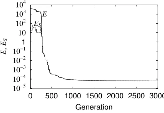
Figure 3 shows one of the successful evolutions of the hy-brid controller when α = 1.0 and β = 1.0. The system is designed for 3000 generations. The squared error ES forms
part of the evaluation function E of the hybrid controller. It is observed that it is relatively small throughout the evo-lution. At 300 generations the running steps error ET = 0,
thus the hybrid is able to control all the state variables of the six trailer-truck system for the maximum running steps from all the patterns. Beyond 300 generations only the squared errors ES are minimized.
10
−510
−410
−310
−210
−11
10
10
210
310
40
500 1000 1500 2000 2500 3000
E,
E
SGeneration
E
E
SFig. 3. Effect of generational training of the NCs on system errors ES, E. (α = 1.0, β = 1.0).
4.3. Control Performance
Figure 4 is an example of the controlled results, for pat-tern no. 9, where the initial orientation and starting vertical position are set to 90 degrees and 6.0m respectively. It is observed that the hybrid controller is able to control the trailer-truck within the training area [-5.0, 10.0]m along x13
successfully.
Figure 5 shows that the hybrid controller optimally con-trols the state variables. Fig. 5 (a) shows variation of the relative angles (x1, x3, x5, x7, x9, x11) and angle of last trailer
x12with running steps. We see that the angles are controlled
-15 -10 -5 0 5 10 15 -15 -10 -5 0 5 10 15
x
13 [m]x
14 [m] Start EndFig. 4. Trajectory for pattern no. 9. Display interval: 140 time steps.
successfully by the hybrid controller design to within the set range [−π/2, π/2] rad. Fig. 5(b) gives the vertical position x13 of the last trailer. It is well within the training range.
Generally, at 300 steps all the state variables are very small and the system eventually realigns and stabilizes at the de-sired path x13=0. -2 -1 0 1 2 0 100 200 300 400 500 600 Angles [rad] Step x1 x3 x5 x7 xx911 x12
(a) Angular differences
-6 -4 -2 0 2 4 6 0 100 200 300 400 500 600 x13 [m] Step
(b) Vertical position of trailer 6 Fig. 5. Variation with running steps
Figures 6(a), (b) and (c) show, respectively, the variation of the LQR, NC and hybrid controller outputs uL(t), uN(t)
and u(t), with running steps. We observe that the LQR output is initially out of range but stabilizes after a while. At about 200 running steps uN(t) is practically zero and
only the LQR is effective. The hybrid output u(t) does not exceed the set range [−π/2, π/2] of the steering angle since the effect of out of range uL(t) is regulated by the NC.
-2 -1 0 1 2 0 100 200 300 400 500 600 uL [rad] Step -2 -1 0 1 2 0 100 200 300 400 500 600 uN [rad] Step (a) LQR, (b) NC -2 -1 0 1 2 0 100 200 300 400 500 600 u [rad] Step (c) Hybrid Fig. 6. Controller outputs
4.4. Control performance for the initial conditions We investigated the workable ranges for both the orien-tation angle and the starting vertical position for the hybrid controller as depicted in Figures 7 and 8. The 3 vertical lines denote the trained initial angles or positions while the Squared error value, 104, refers to the out of control state. In Figure 7, starting vertical position is 3.0m and training values of the angles are 0, π/4, and π/2 rad. It is observed that there is a wider range of untrained start angles [−3π/16, π/2]. Figure 8 shows that the hybrid offers a wider operating range [-3.0, 9.0]m, for the starting vertical position. Orien-tation is π/4 rad and training values are 0.0, 3.0 and 6.0m.
10−6 10−4 10−2 1 102 104 -π/2 0 π/2 π Squared error
Initial angle [rad]
Fig. 7. Control performance for initial angles
10−6 10−4 10−2 1 102 104 -10 -5 0 5 10 15 Squared error
Initial vertical position x13 [m]
Fig. 8. Control performance for initial vertical position
5. Discussion
Table 5 forms the basis of our research. We observe the difficult in designing a controller as the number of trailers increases. Notably, using only the NC fails to control the 6 trailer-truck configuration. Our proposed hybrid controller, comprising the LQR to cater for the linear part and the NC for the nonlinearity, is suitable for the model. The evaluation function of the NC is modified to include both squared errors ESand those due to out of control running steps ET.
For the hybrid system, we designed the LQR and NC con-trollers separately. We optimally chose the best gain factor generated by use of the Riccati equation for the LQR, while for the NC our criterion was based on evaluating both ESand
ET. We used trial and error methods to get the best
combi-nation of the weight matrix W in Eq. (19) for the LQR and the weight q for the NC in Eq. (25). The respective values of weight, 100 for the position magnitude in W and q13 = 0.1
gave the best results in our simulations. Figure 3 shows the sequence of evolution of the hybrid controller when α = 1.0 and β = 1.0. First, ET is successfully minimized, then E is
evaluated by minimizing the squared errors. In case α and β are changed then the evaluation strategy changes.
Figure 4 is representative of the effectiveness of the hy-brid controller in steering the trailer-truck along the desired path from the various starting configurations while backing up. We note from Figure 5(a) and 6 that at 200 steps, all the state variables are relatively small and the NC output grad-ually falls to zero. From this point onward only the LQR is active, thus u(t) = uL(t). The problems of out of control
steering and jack-knife locks are eliminated since all the rel-ative angles are kept to within [−π/2, π/2]rad as per Eqs. (27a) and (27b). We note the superiority of the hybrid con-troller in Figure 6(c), where the output steering angle u(t) oscillates within the desired range [−π/2, π/2]rad.
The neural network property of adaptive learning is sig-nificant in Figures 7 and 8, where extrapolated ranges of op-eration for hybrid are obtained from the three-point training values. Thus even for untrained starting orientation and po-sition, after a while the relative angles are small and thus the system is realigned on the desired trajectory.
The effectiveness of the hybrid concept is demonstrated by the fact that though the complexity of the control problem increases with the number of connected trailers, the combina-tion of the LQR and the NC yield a very powerful controller that operates optimally to execute the trajectory.
6. Conclusion
Our main contribution in this paper is a hybrid control scheme, comprising a LQR and a NC to stabilize the back-ward motion of a six trailer-truck configuration. Motivation for the study stems from the inability of conventional neu-rocontrollers to optimally control the system. Difficult in control is rendered by the nonlinear dynamics of the system and the physical limitations such as jack-knife locks. The system is nonlinear hence the linear system methods are not suitable. Design of the hybrid is based on the condition that we have to include a linearized system for the nonlinear
problem. Our core objective was to design a high perfor-mance controller utilizing neural networks coupled with a linear method. In total the system is able to successfully ex-ecute the manoeuvre to a given trajectory from generic initial conditions while in the backward mode. We have mooted a method that has shown very good performance in control-ling a six trailer-truck configuration. We strongly believe this method may be applied to other nonlinear dynamical control problems.
References
[1] R. Roy, R.K. Pant: “Soft Computing in Engineering De-sign & Manufacturing”. Springer-Verlag London, 1998. [2] M.H. Hassoun: “Fundamentals of Artificial Neural
Net-works”. MIT Press, 1995.
[3] S.A. Harp, T. Samad: “Genetic Synthesis of
Neu-ral Network Architecture”, Handbook of Genetic Al-gorithms, Van Nostrand Reinhold, NY 1991.
[4] K. Tanaka, T. Kosaki: “Fuzzy Backward Movement
Control of a Mobile Robot with Two Trailers”, Trans. of SICE, Vol.33, No.6, pp.541-546, 3/1997 (in Japanese).
[5] K. Tanaka, T. Kosaki, H.O. Wang: “Backing
Con-trol Problem of a Mobile Robot with Multiple Trail-ers: Fuzzy Modeling and LMI-Based Design”, IEEE Transactions on Systems, Man and Cybernetics, Part C, Vol.28, No.3, pp. 329-337, March 1998.
[6] D. Nguyen, B. Widrow: “The Truck Backer-Upper: An
Example of Self-Learning in Neural Networks”, Proceed-ings of the International Joint Conference on Neural Networks (IJCNN-89), Vol.2, pp. 357-363, 1989. [7] R.E. Jenkins, B.P. Yuhas: “A Simplified Neural
Net-work Solution Through Problem Decomposition: The Case of the Truck Backer-Upper”, IEEE Transactions Neural Networks, Vol.4, No.4, pp. 718-720, 1993-4. [8] H. Kinjo, B. Wang, K. Nakazono, T. Yamamoto,
“Back-ward Movement Control of a Trailer-truck System Us-ing Neurocontrollers Evolved by Genetic Algorithms”, Transactions of IEE Japan, Vol.121-C, No.3, pp. 631-641, March 2001 (in Japanese).
[9] B. Wang, H. Kinjo, K. Nakazono, T. Yamamoto:
“De-sign of Backward Movement Control of a Truck System with Two Trailers Using Neurocontrollers Evolved by Genetic Algorithms”, IEEJ Trans. on Electronics, In-formation & Systems, Vol.123, No.5, pp. 983-990, 2003. [10] A. Kiyuna, H. Kinjo, K. Kurata, T. Yamamoto: “Con-trol System Design of Multitrailer Using Neurocon-trollers with Recessive Gene Structure by Step-up GA Training”, IEEJ Transactions on EIS, Vol.125, No.1, pp. 29-36, Jan. 2005 (in Japanese).
[11] P.S. Boyd, H.B. Craig: “Linear Controller Design: Lim-its of Performance”. Prentice-Hall Inc. 1991
[12] G.F. Franklin, J. D. Powell: A. Emami-Naeini, “Feed-back Control of Dynamic Systems”, Prentice Hall. 2002. [13] L.J. Eshelman, D.J. Schaffer: “Real-Coded Genetic Al-gorithms and Interval-Schemata”, Foundations of Ge-netic Algorithms 2, Morgan Kaufmann Publishers, San Mateo, California. pp. 187-202. 1993.