ICCAS2005 June 2-5, KINTEX, Gyeonggi-Do, Korea
A Sliding Surface Design for Linear Systems with Mismatched Uncertainties based on
Linear Matrix Inequality
Seung Ho Jang∗ and Sang Woo Kim∗∗
∗Digital Business Division, SHI Co., Ltd., 493, Banweol-Ri, Taean-Eup, Hwasung-City, Gyeounggi-Do, 445-973, Korea (Tel: +82-31-229-1303; Fax: +82-31-229-1420; Email: [email protected])
∗∗Electrical and Computer Engineering Division, POSTECH, Pohang, 790-784, Korea (Tel: +81-54-279-2237; Fax: +81-54-279-2903; Email: [email protected])
Abstract: Sliding mode control (SMC) is an effective method of controlling systems with uncertainties which satisfy the so-called matching condition. However, how to effectively handle mismatched uncertainties of systems is still an ongoing research issue in SMC. Several methods have been proposed to design a stable sliding surface even if mismatched uncertainties exist in a system. Especially, it is presented that robustness and efficiency of SMC for linear systems with mismatched uncertainties can be improved by reducing mismatched uncertainties in the reduced-order system. The reduction method needs a new sliding surface with an additional component based on Lyapunov redesign technique. In this paper, a stable sliding surface which contains additional component to reduce the influence of mismatched uncertainties, is introduced. It is designed by using linear matrix inequalities that guarantees the stability of the system. A numerical example demonstrates the validity of the proposed scheme.
Keywords: sliding mode control, mismatched uncertainty, linear matrix inequality, robust control
1. Introduction
SMC is an effective method of controlling uncertain systems. Since the system trajectories are constrained on the predeter-mined sliding surfaces in sliding mode, SMC has a good per-formance. The system behavior is insensitive to the internal parameter variations and external disturbances, if uncertain-ties and/or disturbances of the system satisfy the so-called matching condition in this sliding mode. It is possible since uncertainties of the system satisfying the matching condi-tion are completely nullified in sliding mode. Although the system is in sliding mode, the effect of mismatched uncer-tainties of the system remains so that adaptation method, robust method and backstepping method have been used to handle the system with mismatched uncertainties in SMC [1] [3] [4] [5]. Recently, it is shown that robustness and efficiency of SMC for linear systems with mismatched uncertainties can be improved via the reduction of mismatched uncertainties [1].
In sliding mode, an original uncertain system can be changed to the equivalent reduced-order system [7]. Although matched uncertainties are nullified, mismatched uncertainties still re-main in this reduced-order system. Here, mismatched un-certainties can be divided into the matched part, which is in the range space of the input matrix, and the rest part in the reduced-order system [1]. Then, a sliding surface should be designed to nullify the matched part and to stabilize with respect to the rest part.
In this paper, we show a stable sliding surface, which con-tains an additional component to nullify the effect of the match part, can be designed via LMIs if the bound of the rest part satisfies the structured norm bound. A numeri-cal example is given to explain the proposed method and to demonstrate its validity.
This paper is organized as follows: Section 2 briefly intro-duces uncertain systems considered in this paper. In
Sec-tion 3, the sufficient condiSec-tion of stable sliding surface is presented in terms of LMI. Section 4 introduces the reduc-tion method of mismatched uncertainties as well as presents the sufficient condition of new sliding surface with an addi-tional component. In Section 5, sliding mode control law to guarantee a reaching condition is presented. In Section 6, a numerical example is given to illustrate design procedure as well as its validity. Finally, Section 7 serves as a conclusion.
2. Problem statement
Consider the following linear uncertain system:
˙x(t) = (A + ∆A)x(t) + B [(I + ∆B)u(t) + ∆f (t, x)] , (1)
where x ∈ Rn is the state vector, u ∈ Rm is the control
input and ∆ denotes uncertainties. A and B are known constant matrices with appropriate dimensions. Generally, there exists a invertible transformation z = T x such that transforms the system dynamics Eq. (1) to its regular form. Therefore, without loss of generality, the system is described in the regular form such as
· ˙x1 ˙x2 ¸ = · A11 A12 A21 A22 ¸ · x1 x2 ¸ + · ∆A11 ∆A12 0 0 ¸ · x1 x2 ¸ + · 0 B2 ¸ {(I + ∆B2)u + ∆fm} , (2)
where x1 ∈ Rn−m and x2 ∈ Rm are the state vectors,
u ∈ Rm is control input and ∆f
m ∈ Rm represent the
lumped matching uncertainties. ∆A11 and ∆A12 become
mismatched uncertainties. A11, A12, A21, A22 and B2 are
known constant matrices with appropriate dimensions.
Fur-thermore, bounds of ∆fmand ∆B2are assumed to be known.
Assumption 1: Uncertainties ∆fm,∆B2, ∆A11 and ∆A12
are bounded in Euclidean norm by known functions as, ∀(x, t) ∈
Rn×R+, ||∆f
m|| ≤ ρm(x), ||∆B2|| ≤ 1−²band ||∆A11∆A12|| ≤
Assumption 2: The pair (A, B) A = · A11 A12 A21 A22 ¸ , B = · 0 B2 ¸ ,
is controllable, and the matrix B2 has full rank.
Assumption 2 is necessary for the existence of the equivalent control in Section 6.
3. Design of sliding surface using LMI
A linear sliding surface is usually defined as
σ(x) = Sx = 0,
or without loss of generality
σ(x) = ¯Kx =£ K I ¤ · x1 x2 ¸ = 0, (3)
where S ∈ Rm×n and K ∈ Rm×(n−m). In sliding mode,
σ(x) = 0,
x2= −Kx1, (4)
and
˙x1= (A11+ ∆A11)x1− (A12+ ∆A12)Kx1, (5)
which is the reduced-order dynamics. If the uncertainties,
∆A11 and ∆A12, are admissibly norm-bounded and
struc-ture as following:
Assumption 3: Assume that
∆A11= DrFrEr1,
∆A12= DrFrEr2,
where Dr, Er1 and Er2 are known real constant matrices
of appropriate dimensions, and Fr is an unknown matrix
function with Lebesque-measurable elements and satisfies
FT
r Fr≤ I, in which I is the identity matrix.
Under the above condition, the sliding surface Eq. (3), which stabilizes the reduced-order system Eq. (5) in the presence of mismatched uncertainties, can be designed in terms of LMI [3]. In order to show the proof, we need to recall the following matrix inequality.
Lemma 1 [2]: Given constant matrices D and E and a symmetric constant matrix S of appropriate dimensions, the following inequality holds:
S + DF E + ETFTDT < 0,
where F satisfies FTF ≤ R, if and only if for some γ > 0
S + [γ−1ET γD] · R 0 0 I ¸ · γ−1E γDT ¸ < 0.
The main result on the global asymptotic stability of the reduced-order system with mismatched uncertainties is sum-marized in the following theorem.
Theorem 1: If there exist a symmetric and positive
def-inite matrix Pr, some matrix K and some positive γ such
that the following LMI are satisfied, then the reduced-order
system Eq. (5) is asymptotically stabilizable via the sliding mode surface Eq. (3):
Er1QrΨ− Er r2Mr −γI∗ ∗ DT r 0 −γ−1I < 0, (6) where Ψr= QrAT11+ A11Qr− MrTAT12− A12Mr, Qr= Pr−1
and Mr= KPr−1, where * denotes the transposed elements
in the symmetric positions.
Proof: Consider Lyapunov function candidate
V = xT1Prx1, (7)
where Pr is a time-invariant and positive definite matrix.
Clearly, V is positive definite and radially unbounded. The time derivative of V is
˙
V = ˙xT
1Prx1+ xT1Pr˙x1. (8)
By substituting Eq. (5) into Eq. (8), we obtain as follow ˙
V = xT1Φrx1+ xT1(∆A11− ∆A12K)TPrx1
+xT1Pr(∆A11− ∆A12K)x1, (9)
where Φr = AT11Pr+ PrA11− KTAT12Pr− PrA12K. If the
right hand side of Eq. (9) is negative definite uniformly for
all x1 and t ≥ 0 except at x1 = 0 then the reduced-order
dynamics Eq. (5) is asymptotically stable about its zero equilibrium. Therefore, the following inequality is valid.
Φr+ (∆A11− ∆A12K)TPr+ Pr(∆A11− ∆A12K) < 0. (10)
Then, applying Assumption 3 to (10) yields
Φr+ ΣTrFrTDTrP + P DrFrΣr< 0, (11)
where Σr= Er1− Er2K. According to Lemma 1, the matrix
inequality Eq. (11) holds for all Fr satisfying FrTFr ≤ I if
only if there exists a constant γ1/2> 0 such that
Φr+ · γ−1/2Σ r γ1/2(PrDr)T ¸T × · γ−1/2Σ r γ1/2(PrDr)T ¸ = Φr+ · Σr DTPr ¸T· γ−1I 0 0 γI ¸ · Σr DTPr ¸ < 0. (12)
Applying Schur complement to Eq. (12) result in
Φr ∗ ∗ Σr −γI ∗ DT rPr 0 −γ−1I < 0. (13)
Define the following transformation matrix as:
P −1 r 0 0 0 I 0 0 0 I (14)
and take a congruence transformation. This yields
P−1 r ΦrPr−1 ∗ ∗ ΣrPr−1 −γI ∗ DT r 0 −γ−1I < 0. (15)
Denoting Qr = Pr−1 and Mr = KPr−1 yields the LMI Eq.
4. Design of new sliding surface
In this section, a reduced-order dynamics associated with a new sliding surface with an additional component is pre-sented. Additionally, the sufficient condition of new stable sliding surface in terms of LMI is derived. Consider the fol-lowing new sliding surface:
σ(x) = Kx1+ v + x2. (16)
In sliding mode, the reduced-order dynamics will be
˙x1= (A11+ ∆A11)x1− (A12+ ∆A12) {Kx1+ v} . (17)
First of all, mismatched uncertainties ∆A11and ∆A12should
be divided into the matched part, which is in the range space
of A12, and the rest part. That is, Dr should be divide into
the projection on the range space of A12 and the rest such
as
Dr= A12Tp+ ¯Dr.
Therefore, mismatched uncertainties ∆A11 and ∆A12 are
rewritten as follows
∆A11= A12∆A¯ 11+ ∆Aru1, (18)
∆A12= A12∆A¯ 12+ ∆Aru2, (19)
where ¯∆A11= TpFrEr1, ¯∆A12= TpFrEr2, ∆Aru1= ¯DrFrEr1
and ∆Aru2= ¯DrFrEr2. Then, the reduced-order dynamics
Eq. (17) becomes ˙x1= A11x1+ A12 £ −(I + ¯∆A12) {Kx1+ v} +∆frm] + ∆fru, (20) where ∆frm= ¯∆A11x1,
∆fru= ∆Aru1x1− ∆Aru2{Kx1+ v} .
Suppose, as usual, that the uncertainties are admissibly norm-bounded.
Assumption 4: There exists ² > 0 such that || ¯∆A12|| ≤
1−². And, uncertainty ∆frmis norm-bounded as ||∆frm|| ≤
ρrm||x1||.
We define a candidate of Lyapunov function V (x1) mapping
from Rn−m to R such as
V (x1) = xT1P x1, (21)
where P ∈ R(n−m)×(n−m)is a positive definite matrix.
Fur-thermore, suppose the following additional component
v =ρ¯ 2 rm 2²ζA T 12P x1, (22)
where ζ is a positive scalar and ¯ρrm= ρrm+(1−²)||K||. For
simplicity of notation, a new function is defined as follows
w = 2AT12P x1. (23)
Then, the global asymptotic stability of the uncertain reduced-order system Eq. (20) is summarized in the following theo-rem.
Theorem 2: Assume that Assumption 4 is satisfied and the additional surface component v is given such as Eq. (22). If there exist a symmetric and positive definite matrix P, some matrix K and some positive γ and ζ such that the fol-lowing LMIs are satisfied, then the uncertain reduced-order Eq. (20) is asymptotically stabilizable associated with the new sliding mode surface Eq. (16):
Ψ ∗ ∗ ∗ Ω −γI ∗ ∗ ¯ DT r 0 −γ−1I ∗ Q 0 0 −ζ−1I < 0, (24) where Ψ = QAT 11+ AT11Q − MTAT12− A12M , Ω = Er1Q − Er2M − ρ¯ 2 rm 4² ζ −1E r2AT12, Q = P−1 and M = KP−1, and *
denotes the transposed elements in the symmetric positions.
Proof: Consider the time derivative of the Lyapunov
function Eq. (21). ˙ V (x1) = xT1(A11− A12K)TP x1− xT1P (A11− A12K)x1 +2xT 1P A12 ©
−(I + ¯∆A12)v − ¯∆A12Kx1 +∆frm} + 2xT1P ∆fru.(25)
Using Assumption 4 and Eq. (22), the third term of Eq. (25) satisfies the following inequality
2xT1P A12
©
−(I + ¯∆A12)v − ¯∆A12Kx1+ ∆frm ª ≤ −wT(I + ¯∆A 12)v + || ¯∆A12K||||w||||x1|| +ρrm||w||||x1|| ≤ −²¯ρ 2 rm 4²ζ w T w + {(1 − ²)||K|| + ρrm} ||w||||x1|| = − · ρ¯ rm 2 ||w|| ||x1|| ¸T· ζ−1 −1 −1 ζ ¸ · ρ¯ rm 2 ||w|| ||x1|| ¸ +ζ||x1||2 ≤ ζ||x1||2= ζxT1x1. (26)
Therefore, we obtain the following condition from Eq. (25) and Eq. (26) ˙ V (x1) ≤ xT1(A11− A12K)TP x1+ xT1P (A11− A12K)x1 +ζxT1x1+ 2xT1P ∆fru = xT1Φx1+ ζxT1x1+ 2xT1P ¯DrFrEr1x1 −2xT1P ¯DrFrEr2(Kx1+ v),(27) where Φ = AT 11P + P A11− KTAT12P − P A12K. Using Eq. (22), 2xT1P ¯DrFrEr1x1− 2xT1P ¯DrEr2(K +ρ¯ 2 rm 2²ζA T 12P )x1 = xT1P ¯DrFrΣx1+ xT1ΣTFrTD¯rTP x1, (28) where Σ = Er1− Er2K − ρ¯ 2 rm 2² ζ −1E r2AT12P . Therefore, we obtain the following condition from Eq. (27) and Eq. (28)
˙
V (x1) ≤ xT1Φx1+ ζxT1x1+ xT1P ¯DrFrΣx1
+xT1ΣTFrTD¯TrP x1. (29)
If the right hand side of Eq. (29) is negative definite
reduced-order dynamics Eq. (20) is asymptotically stable about its zero equilibrium. Therefore, assume that the fol-lowing inequality is valid.
Φ + ζI + P ¯DrFrΣ + ΣTFrTD¯TrP < 0. (30)
The conversion of Eq. (30) to LMI Eq. (24) follows the procedure in Theorem 1.
5. Sliding mode control
In the previous section, when the uncertain system Eq. (2) was in the sliding mode, the sliding mode surface was de-signed to guarantee the asymptotic stability of the reduced-order system in terms of LMI. Next, we need to find feedback control law u to drive state trajectories of the system onto the sliding surface. This means that the control law is designed to guarantee the existence of sliding mode or the reaching condition. Before proceeding, for notational simplicity, let the proposed sliding surface be redefined as
σ(x) = Kx1+ v + x2 = Kx1+ρ¯ 2 rm 4²ζw + x2 = (K +ρ¯ 2 rm 2²ζA T 12P )x1+ x2= KTx1+ x2, (31) where KT = K +ρ¯ 2 rm 2²ζA T
12P . The feedback control law satis-fying reaching condition is summarized in the following the-orem.
Theorem 3: For the system Eq. (2) satisfying Assump-tion 1 and 2, the following control law is considered:
u = ½ ueq if σ(x) = 0, ueq− ρ(x)||BB2σ(x) 2σ(x)|| if σ(x) 6= 0, (32) where ueq = −B2−1 · KT I ¸ · A11 A12 A21 A22 ¸ x, ρ(x) > (1 − ²b)||ueq|| + η||B −1 2 KT||||x|| + ρm(x) ²b .
Then, the reaching condition of the sliding surface Eq. (31) is satisfied.
Proof: See reference [1].
6. Numerical example
In this section, we give the results of simulation study. Con-sider the following uncertain system which satisfies Assump-tion 1, AssumpAssump-tion 2 and AssumpAssump-tion 3:
˙x =
aa1121+ ∆a+ ∆a1121 aa2212+ ∆a+ ∆a2212 aa2313+ ∆a+ ∆a1323
a31+ ∆a31 a32+ ∆a32 a33+ ∆a33
x + 0 0 1 {(I + ∆B)u + ∆f } , (33) where a11 a12 a13 a21 a22 a23 a31 a32 a33 = 0.1 0.8 0.2 1.2 2.6 0.8 −0.4 1.7 0.6 , · ∆a11 ∆a12 ∆a21 ∆a22 ¸ = · 0.036 −0.03 0.161 −0.12 ¸ · sin πt + 1 −1 − cos πt cos πt ¸ , · ∆a13 ∆a23 ¸ = · 0.036 −0.03 0.161 −0.012 ¸ · sin πt 0 ¸ , ∆a31 ∆a32 ∆a33 = 0.03 + 0.14 sin 2πt 0 0.19 cos 1.3πt , ∆B = 0.1 cos 1.5πt, ∆f = 0.7 sin 2πt + 0.4. In sliding mode, the reduced-order dynamics of Eq. (33) can be described as · ˙x1 ˙x2 ¸ = · 0.1 0.8 1.2 2.6 ¸ · x1 x2 ¸ + · ∆a11 ∆a12 ∆a21 ∆a22 ¸ · x1 x2 ¸ + · 0.2 0.8 ¸ x3+ · ∆a13 ∆a23 ¸ x3. (34)
In the reduced-order dynamics, mismatched uncertainties can be decomposed such as
· ∆a11 ∆a12 ∆a21 ∆a22 ¸ = DrFrEr1, · ∆a13 ∆a23 ¸ = DrFrEr2, where Dr= · 0.036 −0.03 0.161 −0.12 ¸ , Er1= · 1 0 −1 1 ¸ , Fr= · sin πt −1 0 cos πt ¸ , Er2= · 1 0 ¸ .
Also, Drshould be divided into the projection on
£
0.2 0.8 ¤T
and the rest as follows
Dr= · 0.2 0.8 ¸ [0.2 − 0.15] + · −0.004 0 0.001 0 ¸ .
The sliding surface should be designed by Theorem 2 under the given conditions that:
P = · 3.1514 0.0315 0.0315 3.9924 ¸ , K = · 3.0595 13.1628 ¸T , ζ = 1.1643.
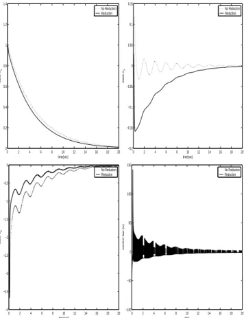
In Figure 1, we compared with the simulation results of the sliding mode controllers which are associated with the slid-ing surfaces designed by Theorem 1 and Theorem 2, respec-tively. simulation results show that if mismatched uncer-tainties are split, the distortion, which is occurred by mis-matched uncertainties,is more considerably decreased. This clearly demonstrates the robustness improvement of reduc-tion of mismatched uncertainties over no-reducreduc-tion of it. This result means that the robustness of the proposed method is better than no reduction method.
7. Conclusion
A new design method of the sliding surface for linear systems with mismatched uncertainties is proposed. This scheme en-ables us to handle mismatched uncertainties by means of offering compensation for the matched part which is in the
range space of the input channel of the reduced-order sys-tems. Additionally, the stabilizing criteria of sliding surface was formulated in terms of LMI. Furthermore, effectiveness of the proposed method is demonstrated by a numerical ex-ample. 0 2 4 6 8 10 12 14 16 18 20 0 0.2 0.4 0.6 0.8 1 1.2 1.4 time(sec) state x 1 No Reduction Reduction 0 2 4 6 8 10 12 14 16 18 20 −0.2 −0.15 −0.1 −0.05 0 0.05 0.1 0.15 time(sec) state x 2 No Reduction Reduction 0 2 4 6 8 10 12 14 16 18 20 −4 −3.5 −3 −2.5 −2 −1.5 −1 −0.5 0 time(sec) state x 3 No Reduction Reduction 0 2 4 6 8 10 12 14 16 18 20 −100 −50 0 50 100 150 time
control law (u)
No Reduction Reduction
Fig. 1. Simulation results of mismatched uncertainty reduc-tion and noreducreduc-tion
References
[1] S. H. Jang and S. W. Kim, “A New Sliding Surface
De-sign Method of Linear Systems with Mismatched Un-certainties,” IEICE Trans. on Fundamentals of
Elec-tronics, Communications and Computer Sciences, vol.
E88-A, No. 1, pp. 387–391, 2005.
[2] H. J. Lee, J. B. Park and C. Chen, “Robust Fuzzy
Con-trol of Nonlinear Systems with Parametric Uncertain-ties,”, IEEE Trans. on Fuzzy Systems, vol. 9, no. 2, pp. 369–379, 2001.
[3] H. H. Choi, “A new method for variable structure
control system design: A linear matrix inequality ap-proach,” Automatica, vol. 33, pp. 2089–2092, 1997.
[4] K.-K. Shyu, Y. -W. Tsai and C. -K. Lai, “Sliding mode
control for mismatched uncertain systems,” Electronics
Letters, vol. 34, no. 24, pp. 2359–2360, 1998.
[5] Chi-Man Kwan, “Sliding mode control of linear systems
with mismatched uncertainties,” Automatica, vol. 31, no. 2, pp. 303–307, 1995.
[6] J. J. E. Slotine and W. Li, Applied Nonlinear Control,
Englewood Cliffs, New Jersey:Prentice-Hall, 1991.
[7] R. A. DeCarlo, S. H. Zak and G.P. Matthews, “Variable
structure control of nonlinear multivariable systems:a Tutorial,” Proceedings of the IEEE, vol. 76, no. 3, pp. 212–232, March 1988.