Copyright ⓒ The Korean Society for Aeronautical & Space Sciences Received: June 13, 2017 Revised: October 30, 2017 Accepted: November 6, 2017
729 http://ijass.org pISSN: 2093-274x eISSN: 2093-2480
Paper
Int’l J. of Aeronautical & Space Sci. 18(4), 729–739 (2017) DOI: http://dx.doi.org/10.5139/IJASS.2017.18.4.729
Minimum-Energy Spacecraft Intercept on Non-coplanar Elliptical Orbits
Using Genetic Algorithms
Snyoll Oghim*, Chang-Yull Lee**, and Henzeh Leeghim***
Chosun University, Gwangju, 61452, Republic of Korea.
Abstract
The objective of this study was to optimize minimum-energy impulsive spacecraft intercept using genetic algorithms. A mathematical model was established on two-body system based on f and g solution and universal variable to address spacecraft intercept problem for non-coplanar elliptical orbits. This nonlinear problem includes many local optima due to discontinuity and strong nonlinearity. In addition, since it does not provide a closed-form solution, it must be solved using a numerical method. Therefore, the initial guess is that a very sensitive factor is needed to obtain globally optimal values. Genetic algorithms are effective for solving these kinds of optimization problems due to inherent properties of random search algorithms. The main goal of this paper was to find minimum energy solution for orbit transfer problem. The numerical solution using initial values evaluated by the genetic algorithm matched with results of Hohmann transfer. Such optimal solution for unrestricted arbitrary elliptic orbits using universal variables provides flexibility to solve orbit transfer problems.
Key words: Two-impulse intercept, Minimum-energy, Non-coplanar elliptic orbit, Genetic algorithm
1. Introduction
Transferring between two positions in space on different orbits is a fundamental problem in orbital mechanics. Obtaining a solution for such orbit transfer problem known as Lambert problem [1] is not simple because many variables need to be considered. The Lambert problem is defined as a problem of finding velocity of a position based on the initial and final positions and time-of-flight.
Many space missions for orbit transfer problems are linked deeply to the Lambert problem. While the Lambert problem generally starts with fixed transfer time and two position vectors, an energy minimum closed-form solution to obtain an orbit for two fixed positions has been evaluated mathematically using geometrical approach or optimization technique [2]. In this approach, the transfer time is a state variable to be obtained for minimum orbital energy.
Efficient use of energy or fuel of spacecraft in space missions is one of the most critical issues because it is directly related to the lifetime of a spacecraft. If energy consumed can
be minimized, it will help engineers to design a spacecraft more efficiently which will save development cost. The orbit transfer problem for spacecraft intercept with minimum energy or fuel has been extensively studied for a long time. Numerous attentions have been paid to this problem due to its importance for space missions [3, 4]. One of the most representative examples is Hohmann transfer for moving between two different circular orbits in the same plane for cost effectiveness. Optimal multiple-impulse time-fixed rendezvous have been extensively studied for low-impulse thrusters. In addition, various constraints or options have been considered [5-7]. Some strategies for safety-optimal linearized impulsive rendezvous for mission success [8] and optimal spacecraft rendezvous using random search algorithms such as genetic algorithm have been studied to overcome numerical problems [9, 10]
Many studies in the literature focusing on spacecraft intercept problems provided by the Lambert algorithm have been restricted by circular or near-circular orbit or coplanar for elliptical orbit cases. Therefore, the intercept problem of
This is an Open Access article distributed under the terms of the Creative Com-mons Attribution Non-Commercial License (http://creativecomCom-mons.org/licenses/by- (http://creativecommons.org/licenses/by-nc/3.0/) which permits unrestricted non-commercial use, distribution, and reproduc-tion in any medium, provided the original work is properly cited.
* Graduate Student, Dept. of Aerospace Engineering
** Assistant Professor, Dept. of Aerospace Engineering
*** Associate Professor, Corresponding author: h.leeghim@controla.re.kr, Dept. of Aerospace Engineering.
DOI: http://dx.doi.org/10.5139/IJASS.2017.18.4.729 730 Int’l J. of Aeronautical & Space Sci. 18(4), 729–739 (2017)
spacecraft considering minimum-energy was addressed for fully three-dimensional elliptic orbits in this study. In fact, there are some computational burden to apply inverse squares equation of motion of spacecraft in elliptical orbit to propagate the position and velocity of a spacecraft. To accurately obtain navigation information at the perigee or apogee, the step size of the numerical integration technique needs to be small. It is obvious that the relative small step size will increase the numerical burden dramatically to obtain sufficiently accurate orbital information of spacecraft on certain time of flight. To adequately manage the numerical burden and difficulties for high elliptical orbits, f and g solution (sometimes called Lagrange coefficients) and universal variables were applied for orbit propagation of spacecraft in this study. The formulation of orbital mechanics by universal variables was produced to resolve difficulty in obtaining numerically accurate position of planet sufficiently in high elliptical orbit.
Many studies have investigated orbit transferring based on the Lambert problem, assuming that there are limited constraints such as coplanar, circle-to-circle, and so on. These assumptions can restrict missions of performing orbit transfer. Therefore, general orbit transfer problems in non-coplanar and elliptic-to-elliptic orbit transfer have been evaluated [11, 12]. Due to strong nonlinearities and discontinuity caused by periodic orbital motion of spacecraft, it is very difficult to obtain a global solution numerically with an initial guess of the Lambert problem in high elliptical orbit. The local minimum makes it hard to find a global solution to the optimization problem. This means that gradient-based numerical search technique is sensitive to initial values. To obtain a global solution, it is necessary to start proper initial values corresponding to the global solution. The key idea in this paper was to use genetic algorithm (GA) (one of global search algorithms [13]) instead of trial-and-error to have the initial value of numerical analysis. This method can reduce computational burdens in trial-and-error. Using this method, the performance index can be minimized more than that obtained through trial-and-error. Therefore, GA plays an important role in finding the initial guess for gradient-based searching algorithm to obtain the optimal value. Finally, the minimum-energy spacecraft intercept for three-dimensional elliptical orbits can be evaluated and accomplished by applying universal variables to resolve numerical difficulties for elliptical orbit. The genetic algorithm can also be used for searching for optimal global energy solution under high nonlinear constraints provided with certain search area.
The remainder of this paper is organized as follows. In Section 2, we briefly reviewed Kepler’s time-of-flight equation based on universal variable and f and g solution.
A necessary condition (so called intercept condition for minimum energy spacecraft intercept strategy) is then introduced by the optimization technique. GA is presented in Section 3 to search for global solution in a given search area. Next, numerical optimization strategies for solving intercept problems by applying GA are addressed in section 4. Three numerical examples for minimum-energy spacecraft intercept on elliptical orbits are addressed in Section 5. To guarantee that the suggested technique provides correct solution, the optimal solution provided by the proposed algorithm is firstly compared with resultant value of Hohmann transfer. Three-dimensional elliptical orbit transfer problems for spacecraft intercept are then followed. Finally, concluding remarks are provided in Section 6.
2. Minimum-energy spacecraft intercept
problem
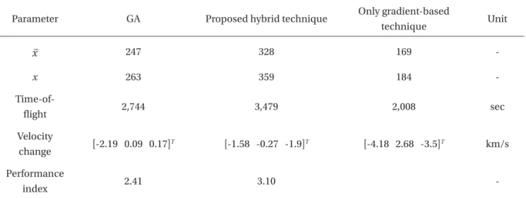
The definition of minimum-energy spacecraft intercept problem is addressed in this section. An initial condition for this problem is the known position and velocity vectors of two spacecraft (i.e., target and interceptor). Fig. 1 shows the overall definition of the problem. In this figure,
5
Fig. 1. Geometry of the minimum energy problem.
in a given search area. Next, numerical optimization strategies for solving intercept problems by applying GA are addressed in section 4. Three numerical examples for minimum-energy spacecraft intercept on elliptical orbits are addressed in Section 5. To guarantee that the suggested technique provides correct solution, the optimal solution provided by the proposed algorithm is firstly compared with resultant value of Hohmann transfer. Three-dimensional elliptical orbit transfer problems for spacecraft intercept are then followed. Finally, concluding remarks are provided in Section 6.
2. Minimum-energy spacecraft intercept problem
The definition of minimum-energy spacecraft intercept problem is addressed in this section. An initial condition for this problem is the known position and velocity vectors of two spacecraft (i.e., target and interceptor). Figure 1 shows the overall definition of the problem. In this figure, ���, ���, ��, and �� represent the initial position and velocity vectors of target and interceptor, respectively. Finally, finding the minimum
,
5
Fig. 1. Geometry of the minimum energy problem.
in a given search area. Next, numerical optimization strategies for solving intercept problems by applying GA are addressed in section 4. Three numerical examples for minimum-energy spacecraft intercept on elliptical orbits are addressed in Section 5. To guarantee that the suggested technique provides correct solution, the optimal solution provided by the proposed algorithm is firstly compared with resultant value of Hohmann transfer. Three-dimensional elliptical orbit transfer problems for spacecraft intercept are then followed. Finally, concluding remarks are provided in Section 6.
2. Minimum-energy spacecraft intercept problem
The definition of minimum-energy spacecraft intercept problem is addressed in this section. An initial condition for this problem is the known position and velocity vectors of two spacecraft (i.e., target and interceptor). Figure 1 shows the overall definition of the problem. In this figure, ���, ���, ��, and �� represent the initial position and velocity vectors of target and interceptor, respectively. Finally, finding the minimum
, and
5
Fig. 1. Geometry of the minimum energy problem.
in a given search area. Next, numerical optimization strategies for solving intercept problems by applying GA are addressed in section 4. Three numerical examples for minimum-energy spacecraft intercept on elliptical orbits are addressed in Section 5. To guarantee that the suggested technique provides correct solution, the optimal solution provided by the proposed algorithm is firstly compared with resultant value of Hohmann transfer. Three-dimensional elliptical orbit transfer problems for spacecraft intercept are then followed. Finally, concluding remarks are provided in Section 6.
2. Minimum-energy spacecraft intercept problem
The definition of minimum-energy spacecraft intercept problem is addressed in this section. An initial condition for this problem is the known position and velocity vectors of two spacecraft (i.e., target and interceptor). Figure 1 shows the overall definition of the problem. In this figure, ���, ���, ��, and �� represent the initial position and velocity vectors of target and interceptor, respectively. Finally, finding the minimum represent the initial position and velocity vectors of target
and interceptor, respectively. Finally, finding the minimum velocity change,
6
velocity change, ���, at a given initial position of interceptor is the main objective to hit the target spacecraft.
To understand problems discussed in this paper, Kepler's equation is now introduced. The � and � solution and universal variable are briefly reviewed. First, the well-known Kepler's equation is described below:
sin
M E e E , (1)
where � is the mean anomaly and � and � represent eccentric anomaly and eccentricity, respectively.
The Kepler's equation has a property that the accuracy of computation becomes lower when the eccentricity approaches unity. To overcome numerical issue, universal variable is proposed. By using this new variable, the governing equations of motion of spacecraft with respect to the position and time-of-flight of spacecraft are given by the following [1]:
0 0
0
sin x T 1 cos x sin x
t a x a a r a a a a r v , (2) 0 0T sin x r0 1 cos x r a a a a a a r v , (3)
where � means the gravitational constant of the earth, � means the position of the spacecraft, � is time-of-flight, � is semi-major axis of orbit of spacecraft, �� and �� represent the initial position and velocity of the spacecraft, respectively, and � is the universal variable defined as √� �⁄ [1]. By using Eq. (2), the universal Kepler's equation of spacecraft can be obtained as follows:
0 01 , sin 1 cos 0 sin
T x x x x t a x a a r a t a a a r v , (4)
, at a given initial position of interceptor is the main objective to hit the target spacecraft.
To understand problems discussed in this paper, Kepler’s equation is now introduced. The f and g solution and universal variable are briefly reviewed. First, the well-known Kepler’s equation is described below:
6
velocity change, ���, at a given initial position of interceptor is the main objective to hit the target spacecraft.
To understand problems discussed in this paper, Kepler's equation is now introduced. The � and � solution and universal variable are briefly reviewed. First, the well-known Kepler's equation is described below:
sin
M E e E , (1)
where � is the mean anomaly and � and � represent eccentric anomaly and eccentricity, respectively.
The Kepler's equation has a property that the accuracy of computation becomes lower when the eccentricity approaches unity. To overcome numerical issue, universal variable is proposed. By using this new variable, the governing equations of motion of spacecraft with respect to the position and time-of-flight of spacecraft are given by the following [1]:
0 0
0
sin x T 1 cos x sin x
t a x a a r a a a a r v , (2) 0 0T sin x r0 1 cos x r a a a a a a r v , (3)
where � means the gravitational constant of the earth, � means the position of the spacecraft, � is time-of-flight, � is semi-major axis of orbit of spacecraft, �� and �� represent the initial position and velocity of the spacecraft, respectively, and � is the universal variable defined as √� �⁄ [1]. By using Eq. (2), the universal Kepler's equation of spacecraft can be obtained as follows:
0 01 , sin 1 cos 0 sin
T x x x x t a x a a r a t a a a r v , (4) , (1)
where M is the mean anomaly and E and e represent eccentric anomaly and eccentricity, respectively.
5
Fig. 1. Geometry of the minimum energy problem.
in a given search area. Next, numerical optimization strategies for solving intercept problems by applying GA are addressed in section 4. Three numerical examples for minimum-energy spacecraft intercept on elliptical orbits are addressed in Section 5. To guarantee that the suggested technique provides correct solution, the optimal solution provided by the proposed algorithm is firstly compared with resultant value of Hohmann transfer. Three-dimensional elliptical orbit transfer problems for spacecraft intercept are then followed. Finally, concluding remarks are provided in Section 6.
2. Minimum-energy spacecraft intercept problem
The definition of minimum-energy spacecraft intercept problem is addressed in this section. An initial condition for this problem is the known position and velocity vectors of two spacecraft (i.e., target and interceptor). Figure 1 shows the overall definition of the problem. In this figure, ���, ���, ��, and �� represent the initial position and
velocity vectors of target and interceptor, respectively. Finally, finding the minimum Fig. 1. Geometry of the minimum energy problem.
731
Snyoll Oghim Minimum-Energy Spacecraft Intercept on Non-coplanar Elliptical Orbits Using Genetic Algorithms
http://ijass.org
7
0
0 0
2 , , 0 sin 1 cos 0 sin
T x x x x t a x a a r a t a a a r v v v , (5)
where �� is the orbital motion of target spacecraft and �� is the equation of motion of the interceptor in orbit.
The position and velocity of the two spacecraft at time-of-flight � can be expressed using � and � solution as below:
0 0 f r r g , v (6) 0 0 f v r g , v (7)
where �, �, ��, and �� are defined as 0 1 a 1 cos x f r a , (8) sin a x t x a a g , (9) 0 sin a x f rr a , (10) 1 a 1 cos x r a g , (11)
In addition, � and � solutions satisfy the following: 1
fgfg , (12)
Next, an optimization technique to obtain a proper solution to minimum-energy intercept problem is necessary. The performance index, �, for orbital energy in this orbit problem can be augmented to a quadratic form of velocity change [2]. Therefore, the cost function for this energy-minimum spacecraft intercept problem is defined as
0 0 1 2 T
J v v , (13)
The Kepler’s equation has a property that the accuracy of computation becomes lower when the eccentricity approaches unity. To overcome numerical issue, universal variable is proposed. By using this new variable, the governing equations of motion of spacecraft with respect to the position and time-of-flight of spacecraft are given by the following [1]:
6
velocity change, ���, at a given initial position of interceptor is the main objective to hit the target spacecraft.
To understand problems discussed in this paper, Kepler's equation is now introduced. The � and � solution and universal variable are briefly reviewed. First, the well-known Kepler's equation is described below:
sin
M E e E , (1)
where � is the mean anomaly and � and � represent eccentric anomaly and eccentricity, respectively.
The Kepler's equation has a property that the accuracy of computation becomes lower when the eccentricity approaches unity. To overcome numerical issue, universal variable is proposed. By using this new variable, the governing equations of motion of spacecraft with respect to the position and time-of-flight of spacecraft are given by the following [1]:
0 0
0
sin x T 1 cos x sin x
t a x a a r a a a a r v , (2) 0 0T sin x r0 1 cos x r a a a a a a r v , (3)
where � means the gravitational constant of the earth, � means the position of the spacecraft, � is time-of-flight, � is semi-major axis of orbit of spacecraft, �� and �� represent the initial position and velocity of the spacecraft, respectively, and � is the universal variable defined as √� �⁄ [1]. By using Eq. (2), the universal Kepler's equation of spacecraft can be obtained as follows:
0 01 , sin 1 cos 0 sin
T x x x x t a x a a r a t a a a r v , (4) 6
velocity change, ���, at a given initial position of interceptor is the main objective to hit the target spacecraft.
To understand problems discussed in this paper, Kepler's equation is now introduced. The � and � solution and universal variable are briefly reviewed. First, the well-known Kepler's equation is described below:
sin
M E e E , (1)
where � is the mean anomaly and � and � represent eccentric anomaly and eccentricity, respectively.
The Kepler's equation has a property that the accuracy of computation becomes lower when the eccentricity approaches unity. To overcome numerical issue, universal variable is proposed. By using this new variable, the governing equations of motion of spacecraft with respect to the position and time-of-flight of spacecraft are given by the following [1]:
0 0
0
sin x T 1 cos x sin x
t a x a a r a a a a r v , (2) 0 0T sin x r0 1 cos x r a a a a a a r v , (3)
where � means the gravitational constant of the earth, � means the position of the spacecraft, � is time-of-flight, � is semi-major axis of orbit of spacecraft, �� and �� represent the initial position and velocity of the spacecraft, respectively, and � is the universal variable defined as √� �⁄ [1]. By using Eq. (2), the universal Kepler's equation of spacecraft can be obtained as follows:
0 01 , sin 1 cos 0 sin
T x x x x t a x a a r a t a a a r v , (4) , (2) 6
velocity change, ���, at a given initial position of interceptor is the main objective to hit the target spacecraft.
To understand problems discussed in this paper, Kepler's equation is now introduced. The � and � solution and universal variable are briefly reviewed. First, the well-known Kepler's equation is described below:
sin
M E e E , (1)
where � is the mean anomaly and � and � represent eccentric anomaly and eccentricity, respectively.
The Kepler's equation has a property that the accuracy of computation becomes lower when the eccentricity approaches unity. To overcome numerical issue, universal variable is proposed. By using this new variable, the governing equations of motion of spacecraft with respect to the position and time-of-flight of spacecraft are given by the following [1]:
0 0
0
sin x T 1 cos x sin x
t a x a a r a a a a r v , (2) 0 0T sin x r0 1 cos x r a a a a a a r v , (3)
where � means the gravitational constant of the earth, � means the position of the spacecraft, � is time-of-flight, � is semi-major axis of orbit of spacecraft, �� and �� represent the initial position and velocity of the spacecraft, respectively, and � is the universal variable defined as √� �⁄ [1]. By using Eq. (2), the universal Kepler's equation of spacecraft can be obtained as follows:
0 01 , sin 1 cos 0 sin
T x x x x t a x a a r a t a a a r v , (4) , (3)
where μ means the gravitational constant of the earth, r means the position of the spacecraft, t is time-of-flight, a is semi-major axis of orbit of spacecraft, r0 and v0 represent the
initial position and velocity of the spacecraft, respectively, and x is the universal variable defined as
6
velocity change, ���, at a given initial position of interceptor is the main objective to hit the target spacecraft.
To understand problems discussed in this paper, Kepler's equation is now introduced. The � and � solution and universal variable are briefly reviewed. First, the well-known Kepler's equation is described below:
sin
M E e E , (1)
where � is the mean anomaly and � and � represent eccentric anomaly and eccentricity, respectively.
The Kepler's equation has a property that the accuracy of computation becomes lower when the eccentricity approaches unity. To overcome numerical issue, universal variable is proposed. By using this new variable, the governing equations of motion of spacecraft with respect to the position and time-of-flight of spacecraft are given by the following [1]:
0 0
0
sin x T 1 cos x sin x
t a x a a r a a a a r v , (2) 0 0T sin x r0 1 cos x r a a a a a a r v , (3)
where � means the gravitational constant of the earth, � means the position of the spacecraft, � is time-of-flight, � is semi-major axis of orbit of spacecraft, �� and �� represent the initial position and velocity of the spacecraft, respectively, and � is the universal variable defined as √� �⁄ [1]. By using Eq. (2), the universal Kepler's equation of spacecraft can be obtained as follows:
0 01 , sin 1 cos 0 sin
T x x x x t a x a a r a t a a a r v , (4) [1]. By using Eq. (2), the universal Kepler’s equation of spacecraft can be obtained as follows:
6
velocity change, ���, at a given initial position of interceptor is the main objective to hit the target spacecraft.
To understand problems discussed in this paper, Kepler's equation is now introduced. The � and � solution and universal variable are briefly reviewed. First, the well-known Kepler's equation is described below:
sin
M E e E , (1)
where � is the mean anomaly and � and � represent eccentric anomaly and eccentricity, respectively.
The Kepler's equation has a property that the accuracy of computation becomes lower when the eccentricity approaches unity. To overcome numerical issue, universal variable is proposed. By using this new variable, the governing equations of motion of spacecraft with respect to the position and time-of-flight of spacecraft are given by the following [1]:
0 0
0
sin x T 1 cos x sin x
t a x a a r a a a a r v , (2) 0 0T sin x r0 1 cos x r a a a a a a r v , (3)
where � means the gravitational constant of the earth, � means the position of the spacecraft, � is time-of-flight, � is semi-major axis of orbit of spacecraft, �� and �� represent the initial position and velocity of the spacecraft, respectively, and � is the universal variable defined as √� �⁄ [1]. By using Eq. (2), the universal Kepler's equation of spacecraft can be obtained as follows:
0 01 , sin 1 cos 0 sin
T x x x x t a x a a r a t a a a r v , (4) 6
velocity change, ���, at a given initial position of interceptor is the main objective to hit the target spacecraft.
To understand problems discussed in this paper, Kepler's equation is now introduced. The � and � solution and universal variable are briefly reviewed. First, the well-known Kepler's equation is described below:
sin
M E e E , (1)
where � is the mean anomaly and � and � represent eccentric anomaly and eccentricity, respectively.
The Kepler's equation has a property that the accuracy of computation becomes lower when the eccentricity approaches unity. To overcome numerical issue, universal variable is proposed. By using this new variable, the governing equations of motion of spacecraft with respect to the position and time-of-flight of spacecraft are given by the following [1]:
0 0
0
sin x T 1 cos x sin x
t a x a a r a a a a r v , (2) 0 0T sin x r0 1 cos x r a a a a a a r v , (3)
where � means the gravitational constant of the earth, � means the position of the spacecraft, � is time-of-flight, � is semi-major axis of orbit of spacecraft, �� and �� represent the initial position and velocity of the spacecraft, respectively, and � is the universal variable defined as √� �⁄ [1]. By using Eq. (2), the universal Kepler's equation of spacecraft can be obtained as follows:
0 01 , sin 1 cos 0 sin
T x x x x t a x a a r a t a a a r v , (4) , (4) 7
0
0 0
2 , , 0 sin 1 cos 0 sin
T x x x x t a x a a r a t a a a r v v v , (5)
where �� is the orbital motion of target spacecraft and �� is the equation of motion of the interceptor in orbit.
The position and velocity of the two spacecraft at time-of-flight � can be expressed using � and � solution as below:
0 0 f r r g , v (6) 0 0 f v r g , v (7)
where �, �, ��, and �� are defined as 0 1 a 1 cos x f r a , (8) sin a x t x a a g , (9) 0 sin a x f rr a , (10) 1 a 1 cos x r a g , (11)
In addition, � and � solutions satisfy the following: 1
fgfg , (12)
Next, an optimization technique to obtain a proper solution to minimum-energy intercept problem is necessary. The performance index, �, for orbital energy in this orbit problem can be augmented to a quadratic form of velocity change [2]. Therefore, the cost function for this energy-minimum spacecraft intercept problem is defined as
0 0 1 2 T J v v , (13) 7
0
0 0
2 , , 0 sin 1 cos 0 sin
T x x x x t a x a a r a t a a a r v v v , (5)
where �� is the orbital motion of target spacecraft and �� is the equation of motion of the interceptor in orbit.
The position and velocity of the two spacecraft at time-of-flight � can be expressed using � and � solution as below:
0 0 f r r g , v (6) 0 0 f v r g , v (7)
where �, �, ��, and �� are defined as 0 1 a 1 cos x f r a , (8) sin a x t x a a g , (9) 0 sin a x f rr a , (10) 1 a 1 cos x r a g , (11)
In addition, � and � solutions satisfy the following: 1
fgfg , (12)
Next, an optimization technique to obtain a proper solution to minimum-energy intercept problem is necessary. The performance index, �, for orbital energy in this orbit problem can be augmented to a quadratic form of velocity change [2]. Therefore, the cost function for this energy-minimum spacecraft intercept problem is defined as
0 0 1 2 T J v v , (13) , (5)
where μ1 is the orbital motion of target spacecraft and μ2 is
the equation of motion of the interceptor in orbit.
The position and velocity of the two spacecraft at time-of-flight t can be expressed using f and g solution as below:
7
0
0 0
2 , , 0 sin 1 cos 0 sin
T x x x x t a x a a r a t a a a r v v v , (5)
where �� is the orbital motion of target spacecraft and �� is the equation of motion of the interceptor in orbit.
The position and velocity of the two spacecraft at time-of-flight � can be expressed using � and � solution as below:
0 0 f r r g , v (6) 0 0 f v r g , v (7)
where �, �, ��, and �� are defined as 0 1 a 1 cos x f r a , (8) sin a x t x a a g , (9) 0 sin a x f rr a , (10) 1 a 1 cos x r a g , (11)
In addition, � and � solutions satisfy the following: 1
fgfg , (12)
Next, an optimization technique to obtain a proper solution to minimum-energy intercept problem is necessary. The performance index, �, for orbital energy in this orbit problem can be augmented to a quadratic form of velocity change [2]. Therefore, the cost function for this energy-minimum spacecraft intercept problem is defined as
0 0 1 2 T J v v , (13) , (6) 7
0
0 0
2 , , 0 sin 1 cos 0 sin
T x x x x t a x a a r a t a a a r v v v , (5)
where �� is the orbital motion of target spacecraft and �� is the equation of motion of the interceptor in orbit.
The position and velocity of the two spacecraft at time-of-flight � can be expressed using � and � solution as below:
0 0 f r r g , v (6) 0 0 f v r g , v (7)
where �, �, ��, and �� are defined as 0 1 a 1 cos x f r a , (8) sin a x t x a a g , (9) 0 sin a x f rr a , (10) 1 a 1 cos x r a g , (11)
In addition, � and � solutions satisfy the following: 1
fgfg , (12)
Next, an optimization technique to obtain a proper solution to minimum-energy intercept problem is necessary. The performance index, �, for orbital energy in this orbit problem can be augmented to a quadratic form of velocity change [2]. Therefore, the cost function for this energy-minimum spacecraft intercept problem is defined as
0 0 1 2 T J v v , (13) , (7) where f, g, 7
0
0 0
2 , , 0 sin 1 cos 0 sin
T x x x x t a x a a r a t a a a r v v v , (5)
where �� is the orbital motion of target spacecraft and �� is the equation of motion of the interceptor in orbit.
The position and velocity of the two spacecraft at time-of-flight � can be expressed using � and � solution as below:
0 0 f r r g , v (6) 0 0 f v r g , v (7)
where �, �, ��, and �� are defined as 0 1 a 1 cos x f r a , (8) sin a x t x a a g , (9) 0 sin a x f rr a , (10) 1 a 1 cos x r a g , (11)
In addition, � and � solutions satisfy the following: 1
fgfg , (12)
Next, an optimization technique to obtain a proper solution to minimum-energy intercept problem is necessary. The performance index, �, for orbital energy in this orbit problem can be augmented to a quadratic form of velocity change [2]. Therefore, the cost function for this energy-minimum spacecraft intercept problem is defined as
0 0 1 2 T J v v , (13) , and 7
0
0 0
2 , , 0 sin 1 cos 0 sin
T x x x x t a x a a r a t a a a r v v v , (5)
where �� is the orbital motion of target spacecraft and �� is the equation of motion of the interceptor in orbit.
The position and velocity of the two spacecraft at time-of-flight � can be expressed using � and � solution as below:
0 0 f r r g , v (6) 0 0 f v r g , v (7)
where �, �, ��, and �� are defined as 0 1 a 1 cos x f r a , (8) sin a x t x a a g , (9) 0 sin a x f rr a , (10) 1 a 1 cos x r a g , (11)
In addition, � and � solutions satisfy the following: 1
fgfg , (12)
Next, an optimization technique to obtain a proper solution to minimum-energy intercept problem is necessary. The performance index, �, for orbital energy in this orbit problem can be augmented to a quadratic form of velocity change [2]. Therefore, the cost function for this energy-minimum spacecraft intercept problem is defined as
0 0 1 2 T J v v , (13) are defined as 7
0
0 0
2 , , 0 sin 1 cos 0 sin
T x x x x t a x a a r a t a a a r v v v , (5)
where �� is the orbital motion of target spacecraft and �� is the equation of motion of the interceptor in orbit.
The position and velocity of the two spacecraft at time-of-flight � can be expressed using � and � solution as below:
0 0 f r r g , v (6) 0 0 f v r g , v (7)
where �, �, ��, and �� are defined as 0 1 a 1 cos x f r a , (8) sin a x t x a a g , (9) 0 sin a x f rr a , (10) 1 a 1 cos x r a g , (11)
In addition, � and � solutions satisfy the following: 1
fgfg , (12)
Next, an optimization technique to obtain a proper solution to minimum-energy intercept problem is necessary. The performance index, �, for orbital energy in this orbit problem can be augmented to a quadratic form of velocity change [2]. Therefore, the cost function for this energy-minimum spacecraft intercept problem is defined as
0 0 1 2 T J v v , (13) , (8) 7
0
0 0
2 , , 0 sin 1 cos 0 sin
T x x x x t a x a a r a t a a a r v v v , (5)
where �� is the orbital motion of target spacecraft and �� is the equation of motion of the interceptor in orbit.
The position and velocity of the two spacecraft at time-of-flight � can be expressed using � and � solution as below:
0 0 f r r g , v (6) 0 0 f v r g , v (7)
where �, �, ��, and �� are defined as 0 1 a 1 cos x f r a , (8) sin a x t x a a g , (9) 0 sin a x f rr a , (10) 1 a 1 cos x r a g , (11)
In addition, � and � solutions satisfy the following: 1
fgfg , (12)
Next, an optimization technique to obtain a proper solution to minimum-energy intercept problem is necessary. The performance index, �, for orbital energy in this orbit problem can be augmented to a quadratic form of velocity change [2]. Therefore, the cost function for this energy-minimum spacecraft intercept problem is defined as
0 0 1 2 T J v v , (13) , (9) 7
0
0 0
2 , , 0 sin 1 cos 0 sin
T x x x x t a x a a r a t a a a r v v v , (5)
where �� is the orbital motion of target spacecraft and �� is the equation of motion of the interceptor in orbit.
The position and velocity of the two spacecraft at time-of-flight � can be expressed using � and � solution as below:
0 0 f r r g , v (6) 0 0 f v r g , v (7)
where �, �, ��, and �� are defined as 0 1 a 1 cos x f r a , (8) sin a x t x a a g , (9) 0 sin a x f rr a , (10) 1 a 1 cos x r a g , (11)
In addition, � and � solutions satisfy the following: 1
fgfg , (12)
Next, an optimization technique to obtain a proper solution to minimum-energy intercept problem is necessary. The performance index, �, for orbital energy in this orbit problem can be augmented to a quadratic form of velocity change [2]. Therefore, the cost function for this energy-minimum spacecraft intercept problem is defined as
0 0 1 2 T J v v , (13) , (10) 7
0
0 0
2 , , 0 sin 1 cos 0 sin
T x x x x t a x a a r a t a a a r v v v , (5)
where �� is the orbital motion of target spacecraft and �� is the equation of motion of the interceptor in orbit.
The position and velocity of the two spacecraft at time-of-flight � can be expressed using � and � solution as below:
0 0 f r r g , v (6) 0 0 f v r g , v (7)
where �, �, ��, and �� are defined as 0 1 a 1 cos x f r a , (8) sin a x t x a a g , (9) 0 sin a x f rr a , (10) 1 a 1 cos x r a g , (11)
In addition, � and � solutions satisfy the following: 1
fgfg , (12)
Next, an optimization technique to obtain a proper solution to minimum-energy intercept problem is necessary. The performance index, �, for orbital energy in this orbit problem can be augmented to a quadratic form of velocity change [2]. Therefore, the cost function for this energy-minimum spacecraft intercept problem is defined as
0 0 1 2 T
J v v , (13)
. (11)
In addition, f and g solutions satisfy the following:
7
0
0 0
2 , , 0 sin 1 cos 0 sin
T x x x x t a x a a r a t a a a r v v v , (5)
where �� is the orbital motion of target spacecraft and �� is the equation of motion of the interceptor in orbit.
The position and velocity of the two spacecraft at time-of-flight � can be expressed using � and � solution as below:
0 0 f r r g , v (6) 0 0 f v r g , v (7)
where �, �, ��, and �� are defined as 0 1 a 1 cos x f r a , (8) sin a x t x a a g , (9) 0 sin a x f rr a , (10) 1 a 1 cos x r a g , (11)
In addition, � and � solutions satisfy the following: 1
fgfg , (12)
Next, an optimization technique to obtain a proper solution to minimum-energy intercept problem is necessary. The performance index, �, for orbital energy in this orbit problem can be augmented to a quadratic form of velocity change [2]. Therefore, the cost function for this energy-minimum spacecraft intercept problem is defined as
0 0 1 2 T
J v v , (13)
. (12)
Next, an optimization technique to obtain a proper solution to minimum-energy intercept problem is necessary. The performance index, J, for orbital energy in this orbit problem can be augmented to a quadratic form of velocity change [2]. Therefore, the cost function for this energy-minimum spacecraft intercept problem is defined as
7
0
0 0
2 , , 0 sin 1 cos 0 sin
T x x x x t a x a a r a t a a a r v v v , (5)
where �� is the orbital motion of target spacecraft and �� is the equation of motion of the interceptor in orbit.
The position and velocity of the two spacecraft at time-of-flight � can be expressed using � and � solution as below:
0 0 f r r g , v (6) 0 0 f v r g , v (7)
where �, �, ��, and �� are defined as 0 1 a 1 cos x f r a , (8) sin a x t x a a g , (9) 0 sin a x f rr a , (10) 1 a 1 cos x r a g , (11)
In addition, � and � solutions satisfy the following: 1
fgfg , (12)
Next, an optimization technique to obtain a proper solution to minimum-energy intercept problem is necessary. The performance index, �, for orbital energy in this orbit problem can be augmented to a quadratic form of velocity change [2]. Therefore, the cost function for this energy-minimum spacecraft intercept problem is defined as
0 0 1 2 T
J v v , (13)
. (13)
Note that the solution must satisfy universal Kepler's equations of Eqs. (4), (5). In addition, the position of two spacecraft must meet at the end of the time of flight so that
8
Note that the solution must satisfy universal Kepler's equations of Eqs. (4), (5). In addition, the position of two spacecraft must meet at the end of the time of flight so that ࢘ത ൌ ࢘. The performance index and constraints can be adjoined into one equation by using Lagrange multiplier [14]:
T T
H J η r r , (14)
where ߣ் and ߶் are Lagrange multiplier vectors and ߟ א ࣬ଶ is a vector composed of ߟଵ and ߟଶ. Lagrange multipliers are obtained by partially differentiating Eq. (14) with respected to state variables. Consequently, a necessary condition for intercepting the target spacecraft with minimum velocity change is given by [15].
1 0 0 0 T r h x x t t r r r r v L , (15)
where matrix ࡸ is defined as 2 0 0 0 1 L r x r r v v , (16)
If the interceptor satisfying the intercept condition ݄ meets the target, then it can be concluded that the transfer orbit of interceptor is the trajectory with the minimum energy at a given initial condition.
3. Genetic Algorithm
Genetic algorithm(GA) is a well-known stochastic global search algorithm. The concept of GA was first generated by imitating in part the evolution principle of the natural system. It is a mathematical algorithm used to find the optimal solution by constructing a population (arbitrary chosen potential set of solutions in a search space) and artificially evolving the population. There are three artificial mechanisms for GA
. The performance index and constraints can be adjoined into one equation by using Lagrange multiplier [14]:
8
Note that the solution must satisfy universal Kepler's equations of Eqs. (4), (5). In addition, the position of two spacecraft must meet at the end of the time of flight so that ࢘ത ൌ ࢘. The performance index and constraints can be adjoined into one equation by using Lagrange multiplier [14]:
T T
H J η r r , (14)
where ߣ் and ߶் are Lagrange multiplier vectors and ߟ א ࣬ଶ is a vector composed of ߟଵ and ߟଶ. Lagrange multipliers are obtained by partially differentiating Eq. (14) with respected to state variables. Consequently, a necessary condition for intercepting the target spacecraft with minimum velocity change is given by [15].
1 0 0 0 T r h x x tt r r r r v L , (15)
where matrix ࡸ is defined as 2 0 0 0 1 L r x r r v v , (16)
If the interceptor satisfying the intercept condition ݄ meets the target, then it can be concluded that the transfer orbit of interceptor is the trajectory with the minimum energy at a given initial condition.
3. Genetic Algorithm
Genetic algorithm(GA) is a well-known stochastic global search algorithm. The concept of GA was first generated by imitating in part the evolution principle of the natural system. It is a mathematical algorithm used to find the optimal solution by constructing a population (arbitrary chosen potential set of solutions in a search space) and artificially evolving the population. There are three artificial mechanisms for GA
, (14)
where λT and ϕT are Lagrange multiplier vectors and η∈R2
is a vector composed of η1 and η2. Lagrange multipliers are
obtained by partially differentiating Eq. (14) with respected to state variables. Consequently, a necessary condition for intercepting the target spacecraft with minimum velocity change is given by [15]
8
Note that the solution must satisfy universal Kepler's equations of Eqs. (4), (5). In addition, the position of two spacecraft must meet at the end of the time of flight so that ࢘ത ൌ ࢘. The performance index and constraints can be adjoined into one equation by using Lagrange multiplier [14]:
T T
H J η r r , (14)
where ߣ் and ߶் are Lagrange multiplier vectors and ߟ א ࣬ଶ is a vector composed of ߟଵ and ߟଶ. Lagrange multipliers are obtained by partially differentiating Eq. (14) with respected to state variables. Consequently, a necessary condition for intercepting the target spacecraft with minimum velocity change is given by [15].
1 0 0 0 T r h x x tt r r r r v L , (15)
where matrix ࡸ is defined as
2 0 0 0 1 L r x r r v v , (16)
If the interceptor satisfying the intercept condition ݄ meets the target, then it can be concluded that the transfer orbit of interceptor is the trajectory with the minimum energy at a given initial condition.
3. Genetic Algorithm
Genetic algorithm(GA) is a well-known stochastic global search algorithm. The concept of GA was first generated by imitating in part the evolution principle of the natural system. It is a mathematical algorithm used to find the optimal solution by constructing a population (arbitrary chosen potential set of solutions in a search space) and artificially evolving the population. There are three artificial mechanisms for GA
,
(15)
where matrix L0 is defined as
8
Note that the solution must satisfy universal Kepler's equations of Eqs. (4), (5). In addition, the position of two spacecraft must meet at the end of the time of flight so that ࢘ത ൌ ࢘. The performance index and constraints can be adjoined into one equation by using Lagrange multiplier [14]:
T T
H J η r r , (14)
where ߣ் and ߶் are Lagrange multiplier vectors and ߟ א ࣬ଶ is a vector composed of ߟଵ and ߟଶ. Lagrange multipliers are obtained by partially differentiating Eq. (14) with respected to state variables. Consequently, a necessary condition for intercepting the target spacecraft with minimum velocity change is given by [15].
1 0 0 0 T r h x x tt r r r r v L , (15)
where matrix ࡸ is defined as 2 0 0 0 1 L r x r r v v , (16)
If the interceptor satisfying the intercept condition ݄ meets the target, then it can be concluded that the transfer orbit of interceptor is the trajectory with the minimum energy at a given initial condition.
3. Genetic Algorithm
Genetic algorithm(GA) is a well-known stochastic global search algorithm. The concept of GA was first generated by imitating in part the evolution principle of the natural system. It is a mathematical algorithm used to find the optimal solution by constructing a population (arbitrary chosen potential set of solutions in a search space) and artificially evolving the population. There are three artificial mechanisms for GA
. (16)
If the interceptor satisfying the intercept condition h meets the target, then it can be concluded that the transfer orbit of interceptor is the trajectory with the minimum energy at a given initial condition.
3. Genetic Algorithm
Genetic algorithm(GA) is a well-known stochastic global search algorithm. The concept of GA was first generated by imitating in part the evolution principle of the natural system. It is a mathematical algorithm used to find the
. .