Legged Robot Landing Control using Body Stiffness & Damping

(1)

Legged Robot Landing Control using Body Stiffness & Damping

Sanghak Sung, Youngil Youm & Wankyun Chung

Department of Mechanical Engineering

Pohang University of Science & Technology(POSTECH) Robotics & Bio-Mechatronics Lab.

Abstract— This Paper is about landing control of legged robot. Body stiffness and damping is used as landing strategy of a legged robot. First, we only used stiffness control method to control legged robot landing. Second control method,sliding mode controller and feedback linearization controller is applied to enhance position control performance. Through these control algorithm, body center of gravity behaves like mass with spring & damping in vertical direction on contact regime.

Index Terms — Landing, Stiffness, Damping, Legged Robot

I. INTRODUCTION

Humanoid robot research is one of the most interested areas to robot engineers these days. Until now, rapid im-provements of humanoid technology makes it possible that humanoid can walk, go up and down stairs, co-work with human, even jog and do hazardous work instead of human. Nowadays humanoid researchers endeavor to improve the humanoids which can do work more independently and move faster.

Running or hopping motion realization is more complicated work than walking because there is big impact force from ground when it touches down. And more joint torque or actuator force is required to fulfill this fast motion. Running robots have been studied by Raibert [5].Their hopping robots driven by pneumatic and hydraulic actuators per-formed various actions. Recently, some kinds of robots now become to run or hop with its two legs.

In this paper, we propose a control scheme for legged robot to land safely using body stiffness & damping behavior. On first method, we control posture using only stiffness control scheme. Original idea of using body stiffness & damping is based on our previous work on continuous hopping strategy, stiffness modulation method [3]. In this paper, to make robot behave like spring and damper, we use stiffness control formulation and change it into proper form. In [4], we can find similar method about robot walking. They use a virtual model control to make a biped walk. Selection of virtual model and modification of its value is up to engineer and virtual model is applied on leg module. In our work, we use stiffness control scheme to make whole body move in stiffness & damping behavior. The second control method is using sliding mode controller and feedback

linearization controller to make robot behave like stiffness modulated-fashion. To move like mass with spring-damper behavior, we will solve 2nd order differential equation for spring-mass-damper system. From this equation, we can get desired trajectories.

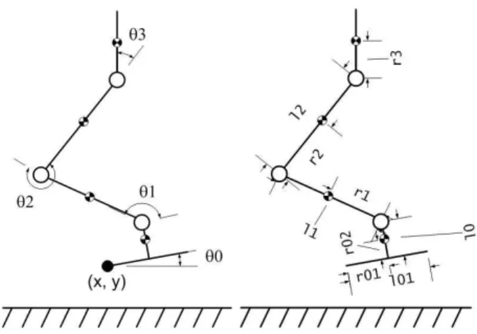
Robot model is in Fig. 1.

Fig. 1. Dimension of the model

Section 2 describes the stiffness modulation method. Section 3 shows stiffness control formulation to use body stiffness and damping in legged robot model and presents dynamic simulation results of legged robot landing. Section 4 shows another control result to enhance position control performance using sliding mode controller and feedback linearization controller.

II. STIFFNESSMODULATIONMETHOD(STIMM) When human hops continually, leg stiffness value in-creases from touch-down to take-off with same initial value on every instant. Below equation is for leg stiffness of human body(leg) when he modulates its value.

k_leg=Fpeak

∆L (1)

(F_peak : peak reaction force in the force platform when human jumps onto that,∆L : vertical displacement of body center of mass)

(2)

Human also uses this leg stiffness modulation on terrain adaptation. It is known that human makes a stiffness adaptation according to change in terrain condition [6].

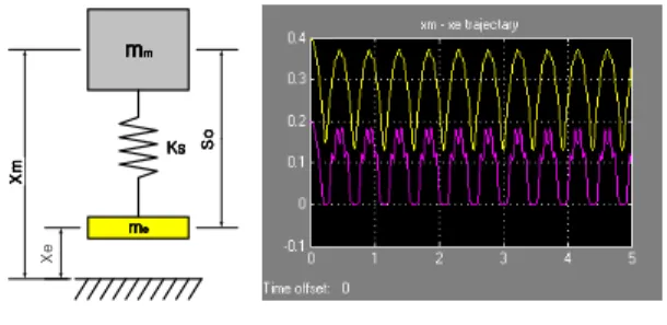
This stiffness modulation method also applied to me-chanical system. In [3], we can see that continuous hopping motion is successful using stiffness modula-tion(Fig 2). Stiffness value of the mechanical system is varied(increased) to compensate energy decrease which comes from impact with ground.

zzzz r r r r

Fig. 2. STIMM on simple model

III. LEGGEDROBOTLANDING USINGSTIFFNESS

CONTROL

To apply body stiffness & damping on legged robot, there needs definition on stiffness and damping value. Simulation model does not have physical spring. So let’s suppose that there is virtual spring element starts from ground and it is attached to the center of gravity point of the model. Through attachment of virtual spring, one can make robot move like mass with spring and damper. All of the profess is confined in contact regime.

A. Attachment of Virtual Spring on Center of Gravity point To express virtual spring attachment, let’s use stiffness control equation.

τ= JT

gFg, (Fg : force from ground) (2) (subscript g and G mean ground point and center of

gravity point respectively)

In above equation, J_gT is defined in local frame {F} in Fig 3, because it is more easy expressing robot’s in-dependent stiffness behavior and it is more natural than expressing in global frame.

To express F_G in the equation, we introduce these relations according to the virtual work theorem.

δX_G= J_Gδθ (3) δXg= Jgδθ (4)

X

G

{F}

{G}

{O}

X

g

Fig. 3. Local coordinate and vectors

δX_G= HδXg, (H = JGJg−1) (5)

Fg= HTF_G (6)

If we insert eqn 6 into eqn 2 and If we use equation which can express stiffness behavior of center of gravity, F_G= K_GδX_G, summarized equation is like this.

τ= JT

gHTKGHJgδθ (7) We can make eqn 7 simple.

τ= JT

GKGJGδθ (8)

Through similar way, damping force also can be im-plemented to the center of gravity. Damping force F_D is defined as

F_D= D_GX˙_G (9)

Resulting torque to the robot is shown below. τ= JT

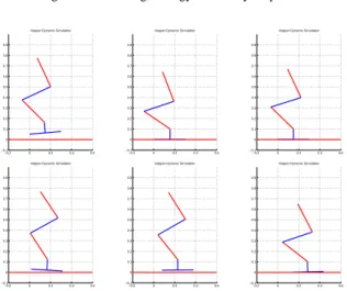
G(FK− FD) (10) From above equation, we can impose stiffness and damping behavior on legged robot. We can try free fall simulation of the robot and the result is in Fig 4, Fig 5. Simulation model has a physical property as, m₀= 0.5kg, m₁= 1.0kg, m₂= 1.0kg, m₃= 3kg, l₀= 0.1m, l₁= 0.3m, l₂= 0.3m, l₃= 0.3m, r₀₁ = 0.1m, r₀₂= 0.05m. Robot’s center of gravity springs out from ground asif it has spring on its end.

When the robot is on contact regime, environment through stiffness control method can be explained as in Fig.(6).

(3)

0 0.5 1 1.5 2 2.5 0 5 10 15 20 25 30 0 0.5 1 1.5 2 2.5 0.34 0.36 0.38 0.4 0.42 0.44 0.46 0.48 0.5 0.52 0.54

Fig. 4. Freefalling, Energy and CG y-displacement

−0.2 0 0.2 0.4 0.6 −0.1 0 0.1 0.2 0.3 0.4 0.5 0.6 0.7 0.8 0.9

Hopper Dynamic Simulation

−0.2 0 0.2 0.4 0.6 −0.1 0 0.1 0.2 0.3 0.4 0.5 0.6 0.7 0.8 0.9

Fig. 5. Free Falling with Stiffness behavior(time passes rightward)

B. Landing Simulation using Stiffness Control

Landing simulation has been performed. In Fig.(7), we can see the force magnitude on center of gravity in x-, direction due to joint torque. In Fig.(8), first graph shows y-dir. center of gravity displacement on which we can identify apparent spring-damper effect on mass. Robot has settled down on ground and we can see that there was energy decrease because of damping and impact force on foot. Vertical stiffness and damping value was used as 5000(Nm) and 100(Nm/s) respectively

Using only simple stiffness controller on center of gravity, we could make landing motion available. From this simulation, we can see that using only body stiffness and damping behavior, legged robot system can land sta-ble without another position control or force control. In human case, this stiffness and damping behavior is also most prominent phenomenon in hopping or landing from air. Hopping motion is also possible using only stiffness control, but hard to control its posture.

Because of simplicity of controller, we could not control robot posture accurately. Especially, in tracking desired x position center of gravity, there needs too much time. On next section, we will show another controller which uses variable structure controller(sliding mode controller).

Fig. 6. Virtual environment in contact regime

Fig. 7. Force on CG in x-,y- direction

IV. LEGGEDROBOTLANDING USINGSLIDINGMODE

CONTROL

A. Dynamics of Legged Robot in Contact Regime

Modelling and dynamics formulation is first required to formulate controller. Legged robot system can be con-sidered as underactuated system on its contact regime because there arises passive joint between the foot and the ground. We assume here that passive joints have the form in rotational joint, not in the translational joints(no sliding in contact point). This type of underactuated system can be modelled as below equation(Eq.(11)).

· 0 τa ¸ = · Muc Mur Mac Mar ¸ · ¨ qr ¨ qc ¸ + · bu ba ¸ (11) This dynamic system has nonholonomic constraints, which is like Eq.(12).

Mucq¨c+ Murq¨r+ bu= 0 (12) (Subscript a, u, c, and r denote quantities related to the active, passive, controlled and uncontrolled joints respec-tively. Active joint can also be an uncontrolled joint.) B. Dynamic Coupling

The position of an underactuated passive joint cannnot be directly controlled because this joint is not equipped with actuator. The passive joint, however, is dynamically

(4)

Fig. 8. y-dir CG displacement & Energy change −0.2 0 0.2 0.4 −0.1 0 0.1 0.2 0.3 0.4 0.5 0.6 0.7 0.8 0.9 time = 0.01 −0.2 0 0.2 0.4 −0.1 0 0.1 0.2 0.3 0.4 0.5 0.6 0.7 0.8 0.9 time = 0.2 −0.2 0 0.2 0.4 −0.1 0 0.1 0.2 0.3 0.4 0.5 0.6 0.7 0.8 0.9 time = 0.24 −0.2 0 0.2 0.4 −0.1 0 0.1 0.2 0.3 0.4 0.5 0.6 0.7 0.8 0.9 time = 0.33 −0.2 0 0.2 0.4 −0.1 0 0.1 0.2 0.3 0.4 0.5 0.6 0.7 0.8 0.9 time = 0.47 −0.2 0 0.2 0.4 −0.1 0 0.1 0.2 0.3 0.4 0.5 0.6 0.7 0.8 0.9 time = 0.7

Fig. 9. Landing simulation(time passes rightward)

coupled to the active joints because of the presence of non-zero off-diagonal elements in the inertia matrix. In this section, we present the coupling index between the acceleration of the passive joint and the accelerations or torques of the active ones.

1) Acceleration Coupling Index: From Eq.(12), if Muu is invertible, we can write

¨

qu= −Muu−1Muaq¨a− Muu−1bu (13) If we set ¨¯quas ¨qu+ Muu−1bu, we can write Eq.(13) as

¨¯qu= −Muu−1Muaq¨a= Guaq¨a (14) To quantify the coupling between the active and the pas-sive joint, it is natural to think of the singular values of Gua. So the acceleration coupling index of the underactuated legged robot system is

ρα(q) = nu

∏

i=1

σi(Gua) (15)

Acceleration coupling index for proposed legged robot model is in Fig.10. From figure, we can identify that the proposed system’s acceleration of passive joint can be controlled using active joints’ acceleration.

5 10 15 20 25 30 35 5 10 15 20 25 30 35 0 0.5 1 1.5 th2:−180~180deg Acceleration Index for Hopping Robot at th3 = 30 Deg

th1:−180~180deg

Acc. Index

Fig. 10. Acceleration coupling index for legged robot model

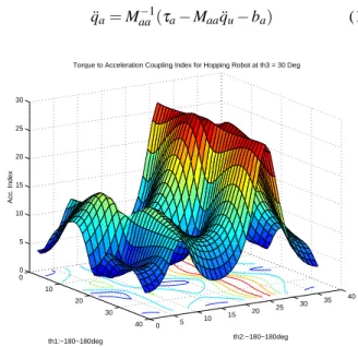
2) Torque to Acceleration Coupling Index: Using sim-ilar process as in acceleration coupling index, we can calculate coupling index between active torque to passive joint’s acceleration(Eq.(16), Fig.11).

¨ qa= Maa−1(τa− Maaq¨u− ba) (16) 0 10 20 30 40 0 5 10 15 20 25 30 35 40 0 5 10 15 20 25 30 th2:−180~180deg Torque to Acceleration Coupling Index for Hopping Robot at th3 = 30 Deg

th1:−180~180deg

Acc. Index

Fig. 11. Torque to acceleration coupling index for legged robot model

C. Feedback Linearization Controller

If we recall Eq.(11), we can reformulate this one into more simple form.

(5)

There are two possible ways of forming the na× 1 vector qc, each one leading to a different strategy for the underactuated legged robot system. First, qc may contain only active joints. When this is the case, we assume all passive joints(joint between the foot and the ground) is locked(i.e foot is full contact condition with ground). This case allows us to control the active joints as if the robot were rooted to the ground(it is an assumption). Second, the vector qc may contain both active and passive joints. According control strategies is shown below as strategy A & AP.

1) Control Strategy A:

τa= Maaq¨a+ ba (17) 2) Control Strategy AP:

τa= (Mac− MarMur−1Muc) ¨qc− MarMur−1bu+ ba (18) Above two control strategies lead to open loop relation-ships between ¨qc andτa of the form,

τa= ¯Macq¨c+ ¯ba (19) Feedback linearization controller(Eq.(20)) now make above system into linear plant.

τa= ¯Macu + ¯ba (20) if ¯Mac is invertible, resulting system is like this

¨

qc= u (21)

D. Robust Control - Sliding Mode Control

In practice, modelling error and eternal disturbances are common. Landing motion also has impact phenomena which is huge disturbance to the system. In this section, we apply robust controller, sliding mode controller, which guarantees asymptotic convergence of the controlled joints to their set points. Because the description of the sliding surface is independent of the system’s kinematic and dy-namic parameters, errors in these quantities do not affect the behavior of the system while in the sliding mode.

Sliding surface is defined like this.

Sc=Γcq˜c+ ˙˜qc (22) According auxiliary input u is chosen as,

u =Γc˙˜qc+ ¨qdc+ Kcsgn(Sc) (23) (where ¨qc is the desired acceleration of the controlled joints, and Γc and Kc are diagonal gain matrices with positive elements.

To avoid chattering in the state trajectory and avoid the excitation of unmodelled high-frequency dynamic compo-nents, we utilize instead the tanh function.

E. Desired path in body stiffness & damping behavior Stiffness control on center of gravity, which was used in previous chapter, did not need desired trajectories because of its simple control form. But, to fulfill accurate motion control on legged robot, we need high level control and accordingly we need desired trajectories for each joints. If whole body mass is m, desired body stiffness is k and desired body damping is d, we can make dynamic equation for mass with spring-damper system.

m ¨y = (y₀− y)k − d ˙y − mg (24) if we reformulate upper equation,

¨ y +d my +˙ k my = y₀k − mg m (25) ¨ y + k₁y + k˙ ₂y = g₁ (26) where (k₁= d/m, k₂= k/m, g₁= (y₀k − mg)/m)) if we solve Eq.(26), y(t) = C₁eλ1t+C 2eλ2 t_{+ g} 1/k2, y(0) = h1, ˙y(0) = h2 (27) λ1,2= −k₁+ − q k2 1− 4k2 2 (28) C₁=h1λ2− h2− g1/k2λ2 λ₂−λ₁ (29) C₂= 1 λ2−λ1 (h₂− h₁λ1+ g1/k2λ1) (30)

Initial condition y(0) and ˙y(0) is assigned as the position and the velocity of center of gravity on initial foot impact on landing. Desired center of gravity trajectory for y(0) = 0.5(m) and ˙y(0) = −1.0(m/s) is in Fig. 12.

F. Landing Simulation using Sliding Mode Control In this section, we apply the controllers provided until now. Overall control diagram is in Fig.14. On initial impact state, nearly all over the cases are point contact(Fig.13(a, b)). So, PA control strategy is first used to control foot joint(θ₀) to zero while another one active joint is not controlled(hip joint, θ₃ in this paper). If passive joint(θ₀) comes to zero(Fig.13(c)), we can apply A control strategy to make robot move in body stiffness & damping behavior. If there is ripple in θ₀ which means point contact state, PA control strategy is applied again to make foot stick to the ground. This PA strategy can be used to make robot’s posture stable from tipping over. From Fig.15, we can

(6)

0 0.2 0.4 0.6 0.8 1 0.38 0.4 0.42 0.44 0.46 0.48 0.5 position path 0 0.2 0.4 0.6 0.8 1 −1.5 −1 −0.5 0 0.5 velocity path 0 0.2 0.4 0.6 0.8 1 −4 −2 0 2 4 6 8 10 acceleration path

Fig. 12. Desired body stiffness & damping path

see that sliding mode controller with feedback lineariza-tion controller shows posilineariza-tion tracking performance in y-direction center of gravity trajectory(Detailed snapshot of simulation is omitted here).

Fig. 13. Contact States (a),(b) : point contact, (C) : full contact

Fig. 14. Control block diagram

V. CONCLUDINGREMARK& FUTUREWORK

In this paper, we tried legged robot landing through two control method. Main idea was using body stiffness &

Fig. 15. y-dir. center of gravity desired & displacement

damping concept to make legged robot land on ground. First, we used stiffness control method, which was simple to apply made good performance about stiffness & damping behavior. But it racked in position control accuracy. In applying sliding mode controller, we developed underactu-ated formulation for legged robot and the controller showed enough position control performance.

To be more natural in landing like human, blending these two control strategies’ advantage is our future work.

REFERENCES

[1] M. Bergerman, Dynamics and control of underactuated manipulators, CMU, Ph.d Dissertation, 1996.

[2] S.Sung, Y.Youm and W.K.Chung, ”Hopping through stiffness modu-lation”, IROS, pp.94-99,2003

[3] F.L.Lewis, C.T.Abdallah and D.M Dawson, Control of robot manip-ulators, MaccMillan Publishing Company, pp.224-245, 1993. x [4] J.Pratt, P.Dilworth and G.Pratt, ”Virtual model control:an intuitive

approach for bipedal locomotion”, IJRR, vel.20, No.2, pp.129-143, Feb. 2001.

[5] M.H.Raibert, Legged robots that balance, MIT Press, 1986 [6] C.T Farley, Han H.P Houdijk, V.Strien and M. Louie,”Mechanism

of leg stiffness adjustment for hopping on surface of diffferent stiffnesses”, APS, Vol.85, No.3, pp.1044-1055,1998.