Available online atwww.sciencedirect.com
ScienceDirect
ICT Express 5 (2019) 235–239
www.elsevier.com/locate/icte
Interference modeling and analysis in 3-dimensional directional UAV
networks based on stochastic geometry
Eunmi Chu
a, Jong Min Kim
b, Bang Chul Jung
a,∗aDepartment of Electronics Engineering, Chungnam National University, Daejeon, South Korea bKorea Science Academy of KAIST, Busan, South Korea
Received 30 August 2019; accepted 16 September 2019 Available online 8 October 2019
Abstract
In this paper, we model and characterize interference of directional unmanned aerial vehicle (UAV) networks based on stochastic geometry, where each UAV is equipped with a directional antenna and it communicates with another UAV that is located in the three dimensional (3D) space. In particular, the 3D location of UAVs is assumed to be uniformly distributed in a certain volume, which is modeled by Poisson point process. Given a beamwidth, we first design an ideal 3D directional antenna beam pattern with a constant gain of both main-lobe and side-lobe. To model the interference in the UAV network, we analyze the effect of elevation and azimuth between a typical UAV receiver and an interfering UAV transmitter with spherical coordinate system. Then, we investigate distribution of the aggregate interference at a typical UAV receiver from multiple UAVs in terms of side-lobe gain, beamwidth, height of UAV, and distance of a UAV transmitter–receiver pair.
c
⃝2019 The Korean Institute of Communications and Information Sciences (KICS). Publishing services by Elsevier B.V. This is an open access article under the CC BY-NC-ND license (http://creativecommons.org/licenses/by-nc-nd/4.0/).
Keywords:UAV networks; Poisson point process (PPP); 3D directional antenna; Interference; Stochastic geometry
1. Introduction
Recently, an unmanned aerial vehicles (UAV) communica-tion has widely been investigated with various applicacommunica-tions due to its low cost of deployment and rapid stabilization of networks. In general, the UAV applications include real-time monitoring of road traffic, remote sensing, disaster communi-cations, product delivery, precision agriculture, etc [1]. Most studies on the UAV communication have focused on per-formance improvement for terrestrial wireless networks. A framework of UAV-assisted vehicular network was introduced in [2], where it was shown that various performance metrics such as connectivity, infrastructure coverage, network infor-mation collection ability, and network interworking efficiency can be improved by cooperating the UAVs and terrestrial communication infrastructure. In [3], coverage probability at a ground user in the UAV-assisted network where multiple UAVs are assumed to be located in a three-dimensional (3D) space and they are assumed to move based on the mixed
∗ Corresponding author.
E-mail addresses: [email protected](E. Chu),[email protected]
(J.M. Kim),[email protected] (B.C. Jung).
Peer review under responsibility of The Korean Institute of Communica-tions and Information Sciences (KICS).
random waypoint mobility model. In [4], a tight lower bound for the outage probability as well as the optimal UAV height for a given air-to-ground link are analytically derived. In [5], a cooperative data dissemination framework was proposed in air-ground integrated networks to maximize the minimum received data amount of ground users, where a terrestrial base station and a single UAV cooperatively serve ground users. In [6], the 3D air–ground channel and 3D antenna patterns between the ground base station and UAV are utilized for more accurate analysis.
Different from UAV-assisted terrestrial wireless networks, a communication among UAVs has not received much attention from both academia and industry due to relatively rare appli-cations and hash technical challenges such as highly mobility of UAVs and frequent topology changes. However, a network consisting of multiple UAVs which are connected by air-to-air wireless channels has recently been investigated due to the increase in the deployment of UAVs. In [7], a novel directional medium access control (MAC) protocol was proposed to coor-dinate transmissions of many UAVs, equipped with directional antennas, in 3D space. Furthermore, an mmWave-enabled UAV swarm network was studied for massive data exchange among UAVs in [8], where a 3D interference graph was https://doi.org/10.1016/j.icte.2019.09.006
2405-9595/ c⃝2019 The Korean Institute of Communications and Information Sciences (KICS). Publishing services by Elsevier B.V. This is an open access article under the CC BY-NC-ND license (http://creativecommons.org/licenses/by-nc-nd/4.0/).
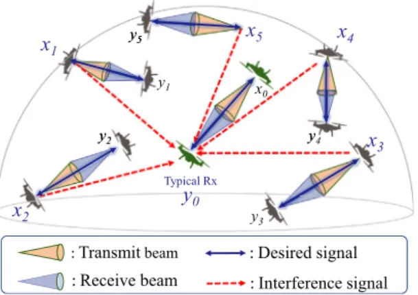
Fig. 1. Directional UAV networks.
exploited by considering mobility, interference, and energy consumption simultaneously.
As the UAV network become denser, the interference among UAV wireless links tends to limit the network per-formance and thus it is important to analyze the interference characteristics of the UAV network in 3D space as shown in
Fig. 1. Existing studies only focused on a simple 3D wireless
network without considering the effect of side-lobe of the directional antennas. In our previous paper [9], we shortly described an ideal 3D directional antenna model consider-ing the effect of side-lobe and then analyze the interference characteristics of the directional UAV network where UAVs are randomly located in 3D space according to Poisson Point Process (PPP).
In this paper, we describe an ideal 3D directional antenna model and a network model in detail. Additionally, we inves-tigate distribution of the aggregate interference at a typical UAV receiver from multiple UAVs in terms of side-lobe, beamwidth, the height of UAV and the distance of a pair of UAV communicating each other.
2. Interference modeling
2.1. Directional antenna model in 3D space
In the ideal omni antenna, the radiation pattern is uniformly radiated to the area of the isotropic sphere. When the radius of sphere is set to 1, surface area Ao is to be 4π. Since the
energy source power Po is radiated on Ao, radiation intensity
Go represents the power radiated from an antenna per unit
sphere and it is expressed as follows: Go=
Po
Ao
, (1)
Assuming that Go is 1, then Po is to be 4π.
In contrast, in the directional antenna, the radiation pattern is consisted of a main-lobe and a side-lobe. Energy source power is separated by the main-lobe and the side-lobe. In directional antenna, the energy source of the omni antenna Po
is expressed as follows:
Po =Pm+Ps, (2)
radiation density of side-lobe Gs is expressed as follows:
Gm= Pm Am (main-lobe), Gs = Ps As (side-lobe). (4)
Since Am is determined by the beamwidth ω, Am(ω) is used
instead of Am as follows:
Am(ω) = ∫ρ=0ω
∫ω
φ=0sinφ dφ dρ, (main-lobe), (5)
where ρ and φ denote azimuth and elevation in a spherical coordinate system, respectively. Similarly, for given ω, the radiation intensity of main-lobe is expressed as follows: Gm(ω) =
Pm(ω)
Am(ω)
, (main-lobe). (6)
The side-lobe is usually radiated to the opposite direction form the main-lobe. It wastes energy and may cause inter-ference to other equipment. All practical antennas incur a certain amount of side-lobe although ideal antennas have zero side-lobe. Let Gs be the radiation intensity of side-lobe, it is
expressed as follows: Gs= Ps As = Po−Pm(ω) Ao−Am(ω) , (side-lobe) , (7)
where the denominator is applied by Eqs.(3)and(5), and the nominator is applied by Eq.(2).
The energy source power of main-lobe for a given ω is calculated from Eq.(7)as follows:
Pm(ω) = Po−Gs(Ao−Am(ω)) . (8)
Therefore, since the gain of main-lobe is calculated by givenω and Gs, Gm(ω) is replaced to Gm(ω, Gs) as follows
Gm(ω, Gs) =
GoAo−Gs(Ao−Am(ω))
Am(ω)
. (9)
In reality, the values of Gm and Gs are varied depending
on the arrival angles. However, for simplicity, we assume an ideal directional antenna gain pattern which are consisted of two constant values of Gs and Gm in this paper.
2.2. Network model in 3D space
We consider a 3-dimensional UAV network where simul-taneously transmitting UAVs are distributed as PPP Γ = {x1, x2, . . .} on R3. Assuming that a terrestrial area is A and
intensity of the UAV on 2-dimensional terrestrial area is λ, the number of UAVs ofλA is distributed on the 3-dimensional UAV network, i.e., the cardinality of Γ isλA. We denote yias
a receiving UAV corresponding to a transmitting UAV xi. We
Fig. 2. UAV’s antenna gain model.
center direction of beamwidthω. The distance between xiand
yi is di which is randomly and uniformly determined within
the range of the minimum distance of dmi n and the maximum
distance of dmax. The value on z-axis of xi, i.e., the height of
UAV hxi also is randomly and uniformly determined within
the range of the minimum height of hmi n and the maximum
height of hmax.
In summary, xi and yi are randomly and uniformly
gener-ated along with the following conditions: xi=(axi, bxi, hxi), yi=(ayi, byi, hyi) on R3,
where ∥xi−yi∥ =di,
dmi n ≤di≤dmax,
hmi n ≤hxi ≤hmax,
hmi n ≤hyi ≤hmax.
A typical receiver yois located in the center of an observing
target area, and the pair of xo and yo also retains the distance
R. To easily calculate antenna gain, we translate the carte-sian coordinate system into the spherical coordinate system. Elevation φ is the angle between the vector of r and the z-axis whereas azimuthρ is the angle between x-axis and the projection of the vector r on the x y plane as shown inFig. 2. The angles (ρxi o, φxi o) and (ρxoi, φxoi) are generated by a vector
of (xi, yo) and a vector of (yo, xi), respectively. Likewise, the
angles (ρo, φo) and (ρi, φi) are generated by their pairs, i.e., a
vector of (yo, xo) and a vector of (xi, yi).
Transmit antenna gain at the typical node yo from
interfer-ence node xiis expressed as follows:
Gt ( ρxi o, φxi o, ω, Gs ) = { Gm(ω, Gs), if (ρxi o ∈ − → Ψi ) ∩(φx i o ∈ − → Φi) , Gs, otherwise, (10) where −→Ψi and − →
Φi denote set of angles of main-lobe for a
pair of xi and yi, i.e.,
− → Ψi = [ ρi−ω2, ρi+ω2 ] and −→Φi = [ φi−ω2, φi+ω2].
Receiver antenna gain at the typical node yo from
interfer-ence node xiis expressed as follows:
Gr ( ρxoi, φxoi, ω, Gs ) = { Gm(ω, Gs), if (ρxoi ∈ ←− Ψi ) ∩(φx oi ∈ ←− Φi) , Gs, otherwise, (11)
Fig. 3. Simplified antenna model of Gm and Gs forω.
where ←Ψ−i and
←−
Φi denote angle of main-lobe for a pair
of xo and yo, i.e., ←− Ψi = [ ρo−ω2, ρo+ω2 ] and ←Φ−i = [ φo−ω2, φo+ω2].
Therefore, the received desired signal S and the inter-ference signal I at the typical receiver yo are expressed as
follows: S = P R−αG m(ω, Gs)Gm(ω, Gs), I = ∑ xi∈Γ Pdi−αGt ( ρxi o, φxi o, ω, Gs) Gr ( ρxoi, φxoi, ω, Gs ) , (12) where Γ denotes the set of interferencing nodes, P denotes transmit power, and di denotes the distance between
interfer-ence nodes and the typical receiver, i.e., di = ∥xi−yo∥. Then,
SINR is expressed as follows:
SINR = S
I +η, (13)
whereη denotes noise power. 3. Simulation results
System parameters are set to R = dmi n = 100 m, α =
2, terrestrial service area A = 10 km × 10 km, the number of UAVs in the terrestrial service area λA = 100, ω = {10◦, 30◦, 60◦, 120◦}, G
s = 0 ∼ 0.2, hmi n = 50 m, hmax =
{150 m, 250 m}, and dmax=100 m ∼ 2000 m. Since the
path-loss exponent for air-to-air was also estimated at 2.05, we consider the free space path-loss exponent of 2 [10].
3.1. The analysis of directional antenna gain
Fig. 3 shows directional antenna gain pattern for varying
Gs andω from Eq.(9). The left plot ofFig. 3shows the gain
of main-lobe for varying Gs andω in dB scale units. As ω is
narrow, the gain of main-lobe increases. Accordingly, as Gs
decreases, the gain of main-lobe increases. Letθ be the angle of the vector from location xi to location yo relative to the
center of beam. If θ is between −ω/2 and ω/2, the antenna gain is Gm(ω), Otherwise Gs. The right plot ofFig. 3 shows
Fig. 4. CDF of aggregate interference according to Gs.
example, atω = 60◦, main-lobe gain of 5 db is achieved from
−30◦ ∼ 30◦ while side-lobe gain of about 0 db is achieved
from −180◦∼ −30◦ and 30◦∼180◦.
3.2. The analysis of CDF of interference
We analyze the interference in terms of the effect of side-lobe gain, beamwidth, and the maximum height. First, we set system parameters to be hmax = 150 m, α = 2, R =
dmi n = dmax = 100 m, and λA = 100. By the condition
of R = dmi n = dmax, a pair of a typical transmitter and
typical receiver retains the distance of R as well as all pairs of interferencing nodes retain the same distance of R.
Fig. 4 shows the CDF of aggregate interference according
to Gs for given ω = 120◦. As Gs increases, the amount
of interference increases due to side-lobe and the CDF of interference is shifted to the right which is the region of strong interference. For no side-lobe of Gs =0, 99% of the nodes
cause small interference amount less than −100 dB.
Fig. 5 shows the CDF of aggregate interference according
toω for given Gs=0.1. In case of an omni antenna, the
aggre-gate interference is between −48 dB and −25 dB. However, for ω = 10◦, the aggregate interference is between −70 db and 8 db. Although 70% of the aggregate interference is less than −65 dB, about 20% cause strong interference greater than −40 dB. Strong interference begins to decrease at 60◦ and there is no overall strong interference at 120◦. Therefore, strong interference cancellation seems to be necessary for the narrow beamwidth.
Fig. 6 shows the CDF of aggregate interference at hmax =
250 m compared to that at hmax = 150 m. In case of an
omni antenna, there is little change in CDF of aggregate interference. When narrow beam likeω = 10◦and wide beam
likeω = 120◦, the strong interference is a little reduced caused
by the increase of the maximum height. Since the narrow beam makes most of strong interference be reduced, the effect of the height increase is negligible. Additionally, since the interference is spread over most of area by wide beam, the effect of the height increase is negligible. At ω = 30◦ and
ω = 60◦, the interference is improved due to increasing
the maximum height. For ω = 30◦, the value of CDF of
Fig. 5. CDF of aggregate interference according toω.
Fig. 6. CDF of aggregate interference according to hmax.
Fig. 7. CDF of aggregate interference according to dmax.
interference at −60 db is increased from 0.4 to 0.55. Also, for ω = 60◦, the value of CDF of interference at −60 db is
increased from 0.15 to 0.35.
Fig. 7 shows the CDF of aggregate interference at dmax =
2000 m compared to that at dmax =100 m for given hmax =
Fig. 8. CDF of SINR according toω.
more reduced caused by the increase of dmax. Forω = 10◦, the
value of CDF of interference at −60 dB is increased from 0.7 to 0.75. Also, forω = 30◦, the value of CDF of interference
at −60 dB is increased from 0.42 to 0.5. However, the CDF of interference slightly is improved atω = 60◦. There is little effect on the increases of dmax in case of ω = 120◦ and an
omni-antenna.
3.3. The analysis of SINR
Fig. 8shows CDF of SINR according toω for given Gs =
0.2, dmax = 100 m, and hmax = 100 m. For small ω, the
antenna gain of the main-lobe is large as shown in Fig. 3. From this, it can be seen that the SINR increases due to a sharp increase in the desired signal. In case ofω = 10◦, SINR
can be seen to increase sharply due to 70% weak interference and the strong desired signal.
4. Conclusions
In this paper, we showed distribution of the aggregate interference and distribution of SINR at a typical UAV receiver from multiple UAVs. From numerical results, we showed that the aggregate interference becomes significantly decreased if the beamwidth decreases or the antenna gain of silobe de-creases. The narrower beamwidth increases the signal strength but it may induce strong interference to other UAV wireless links as well. When the height of UAV increases, the aggre-gate interference become decreased at the beamwidths of 30◦
and 60◦, compared to those of 10◦ and 120◦. Furthermore,
when the distance of a pair of UAV increases, the narrower
beamwidth decreases the aggregate interference. Therefore, interference management techniques and beam steering tech-niques are required for the directional UAV network. We leave the interference management such as interference avoidance or cancellation as well as beam steering finding the space with the least interference for the directional UAV network in a 3D space as a further study.
Acknowledgments
This research was partly supported by the National Re-search Foundation (NRF) of South Korea through the Basic Science Research Program funded by the Ministry of Science and ICT under Grant (NRF2019R1A2B5B01070697) and this research was partly supported by Basic Science Research Program through the NRF funded by the Ministry of Education of South Korea (NRF-2018R1A6A3A01012714).
Conflict of interest
The authors declare that there is no conflict of interest in this paper.
References
[1] H. Shakhatreh, et al., Unmanned aerial vehicles: A survey on civil applications and key research challenges, 2018, arXiv preprintarXiv: 1805.00881.
[2] W. Shi, H. Zhou, J. Li, W. Xu, N. Zhang, X. Shen, Drone assisted vehicular networks: Architecture, challenges and opportunities, IEEE Netw. 32 (3) (2018) 130–137.
[3] P. Sharma, D. Kim, Coverage probability of 3-D mobile UAV networks, IEEE Wireless Commun. Lett. 8 (1) (2019) 97–100.
[4] Z. Yuan, J. Jin, L. Sun, K. Chin, C. Muntean, Ultra-reliable IoT communications with UAVs: A swarm use case, IEEE Commun. Mag. 56 (12) (2018) 90–96.
[5] Z. Xue, J. Wang, G. Ding, Cooperative data dissemination in air-ground integrated networks, IEEE Wireless Commun. Lett. 8 (1) (2019) 209–212.
[6] J. Lyu, R. Zhang, Network-connected UAV: 3D system modeling and coverage performance analysis, IEEE Internet Things J. (2019) arXiv preprintarXiv:1901.07887.
[7] Z. Zheng, A. Sangaiah, T. Wang, Adaptive communication protocols in flying ad hoc network, IEEE Commun. Mag. 56 (1) (2018) 136–142.
[8] Z. Feng, L. Ji, Q. Zhang, W. Li, Spectrum management for mmwave enabled UAV swarm networks: Challenges and opportunities, IEEE Commun. Mag. 57 (1) (2019) 146–153.
[9] E. Chu, J. Kim, B. Jung, Interference analysis of directional UAV networks: A stochastic geometry approach, in: Proc. IEEE ICUFN, Jul. 2019.
[10] N. Ahmed, S. Kanhere, S. Jha, On the importance of link character-ization for aerial wireless sensor networks, IEEE Commun. Mag. 54 (5) (2016) 52–57.