Statistical Signal Processing Algorithms for Radar and Sonar System

(1)

Statistical Signal Processing Algorithms

for Radar and Sonar System

Jeong Hee Han

Department of Oceanic Information and System Engineering

GRADUATE SCHOOL

CHEJU NATIONAL UNIVERSITY

(2)

Statistical Signal Processing Algorithms

for Radar and Sonar System

Jeong Hee Han

(Supervised by Professor Jinho Bae)

A Thesis submitted in partial fulfillment of the requirement for

the degree of Master of Engineering

2009. 2

Department of Oceanic Information and System Engineering

GRADUATE SCHOOL

(3)

(4)

SUMARY

The ocean equipments such as maritime radar and sonar system play a vital role in ship navigation, collision avoidance and ocean investigation. Especially such equipments require great accuracy and reliability. To improve the performance of those equipments, statistical signal processing methods will be required.

Typical maritime radar is used either in the α-β tracker or the Kalman tracker to track moving targets. However, if α and β coefficients are not suitable, the α-β tracker does not guarantee the accuracy of the position and velocity estimation for a non-linear moving target. The Kalman tracker demands the statistical characteristics of the maneuvering targets and it has a heavy computational cost. To solve the problems, the switched slide window tracker (SSWT) using a moving piecewise window was proposed in this study. The proposed algorithm does not require the statistical characteristics of a target and demands low computational cost. To verify the algorithm, the maritime radar simulator with the proposed algorithm is implemented using a TMS320C6711 digital signal processor (DSP) board and LabVIEW 8.5.

In the underwater communications, transmitted acoustic signal is corrupted by interference from multipath. A parametric array transducer is capable of radiating a narrow beam with very low sidelobe levels. In certain cases, the parametric array transducer can help the multipath

(5)

problem. In the thesis, the sonar communication system using the parametric array transducer was presented. To detect the signal without error, the measured signal was averaged for a particular window size before applying the maximum likelihood method.

Our implementation has the potential to improve the performance of the ocean equipments such as radar and sonar system.

(6)

LIST OF FIGURES

Figure 2-1. Attained simulation results of the α-β tracker...15

Figure 2-2. The error curves by the coefficient α ...16

Figure 2-3. Attained simulation results of the α-β tracker...17

Figure 2-4. The error curves by the coefficient α ...18

Figure 2-5. Attained simulation results of the Kalman tracker...22

Figure 2-6. The error curves by the noise covariance ...23

Figure 2-7. Attained simulation results of the Kalman tracker...24

Figure 2-8. The error curves by the noise covariance ...25

Figure 2-9. Flow chart for the SSWT...27

Figure 2-10. A piecewise linear model for non-linear moving target ...28

Figure 2-11. Attained simulation results of the SSWT...31

Figure 2-12. The error curves by the window size...32

Figure 2-13. Attained simulation results of the SSWT ...33

Figure 2-14. The error curves by the window size...34

Figure 2-15. The trajectory of each algorithm...35

Figure 2-16. The error curves of each algorithm ...36

(9)

Figure 2-27. Block diagram of simulator ...50

Figure 2-28. The DSP board...50

Figure 2-29. The maritime radar simulator ...52

Figure 2-30. The maritime radar simulator ...53

Figure 3-1. Measured signal ...59

Figure 3-2. The average value of the signal ...60

Figure 3-3. The probability density function of the signal ...60

Figure 3-4. Block diagram of transmitter...62

(10)

Figure 3-6. Block diagram of receiver ...64

Figure 3-7. The structure of the signal frame ...65

Figure 3-8. (a) The modulated signal and (b) a period of frame measured by oscilloscope ...65

Figure 3-9. The GUI transmitter ...66

(11)

LIST OF TABLES

Table 2-1. The target model for the simulation...14

Table 2-2. Error of the α-β tracker ...16

Table 2-3. Error of the α-β tracker ...19

Table 2-4, Error of the Kalman tracker ...23

Table 2-5. Error of the Kalman tracker ...26

Table 2-6. The weight values...29

Table 2-7. Error of the switched slide window tracker ...32

Table 2-8. Error of each tracking algorithm ...34

Table 2-14. Error of the each tracking algorithm...48

Table 2-15. Specifications of the DSP board...51

Table 3-1. Specifications of PXI-6070E...62

(12)

CHAPTER 1 Introduction

The ocean equipment such as maritime radar and sonar system play a vital role in ship navigation, collision avoidance, ocean investigation and underwater communication [1]. Especially these equipments require great accuracy and reliability [2]. To improve the performance of these equipments, the statistical signal processing method will be required [3].

Typical maritime radar is used either in the α-β tracker or the Kalman tracker to track moving targets [4]. However, if α and β coefficients are not suitable in the case of a non-linear moving target, the accuracy of the position and velocity estimation is not guaranteed [5]. The Kalman tracker demands the statistical characteristics of the maneuvering targets and it has a heavy computational cost [6]. To solve these problems, the switched slide window tracker (SSWT) using a moving piecewise window was proposed in this study [7]. The proposed algorithm does not require the statistical characteristics of a target and demands low computational cost. In addition, our algorithm is more effective than the α-β tracking tracker for a non-linear moving target. To verify the algorithm, the maritime radar simulator with the α-β tracker, the Kalman tracker and the proposed algorithm is implemented using a TMS320C6711 digital signal processor (DSP) board and LabVIEW 8.5 [8] [9].

(13)

from multipath [10]. A parametric array transducer is capable of radiating a narrow beam with very low sidelobe levels [11]. In certain cases, the parametric array transducer can help the multipath problem. In the thesis, the sonar communication system using the parametric array transducer was presented. To detect the signal without error, the measured signal was averaged for a particular window size before applying the maximum likelihood method [12]. The graphic user interface (GUI) control programs for the sonar communication system are developed by LabVIEW 8.5, which can be modified easily.

Chapter 2 presents the maritime radar simulator using the proposed tracking algorithm. Chapter 3 presents the parametric array sonar system using the prototype parametric array transducer. Finally, Chapter 4 describes some of the research results.

(14)

CHAPTER 2 The Maritime Radar Simulator

2.1 Introduction

Maritime radar and sonar system play a vital role in ship navigation, collision avoidance [1]. Typical maritime radar is a track while scan (TWS) radar, which is used either in the α-β tracker or the Kalman tracker to track moving targets [4].

In cases where the statistical characteristics of the maneuvering targets are known exactly, the Kalman tracker gives an excellent tracking performance [13]. However, it is difficult to find the statistical characteristics of the maneuvering target in advance. Furthermore, the Kalman tracker has a heavy computational cost [6].

The α-β tracker is more popular than the Kalman tracker because of its simplicity and it does not demand high computational cost [7]. However, if α and β coefficients for non-linear moving target are not suitable for a non-linear moving target, the accuracy of the position and velocity estimation is not guaranteed [5].

To solve these problems, the switched slide window tracking (SSWT) algorithm using a moving piecewise window was proposed in the thesis [7]. The proposed algorithm does not require prior statistical characteristics of a target and demands low computational cost. In addition, the proposed algorithm is more effective than the α-β tracking tracker for non-linear

(15)

moving targets.

To verify the algorithm, the maritime radar simulator with the α-β tracker, the Kalman tracker and the SSWT is implemented using a TMS320C6711 digital signal processor (DSP) board [8] [9]. The simulator is used to track and display the moving target, and it has graphic user interface (GUI).

Section 2.2 gives a brief overview of the different algorithms used in the α-β tracker, the Kalman tracker and the proposed tracker. Section 2.3 presents the maritime radar simulator using the proposed algorithm. Finally, Section 2.4 describes some of the research results.

(16)

2.2 Conventional Algorithms

2.2.1 The α-β Tracker

The α-β tracker is used for tracking targets. The α-β tracker is defined as

( ) ( ) ( ) ( ) , ( ) ( ) / ( ) ( ) , ( 1) ( ) ( ) , ( 1) ( ), F p m p F p m p p F F p F x k x k x k x k V k V k T x k x k x k x k V k T V k v k

a

b

é ù = + _ë - _û é ù = + _ë - _û + = + + = (2-1)

where x_m(k) is the

x

coordinate of the target’s measured position, x_p(k) is the

x

coordinate of the target’s predicted position, V_p(k) is the predicted target velocity in the

x

direction,

x k

_F

( )

is the

x

coordinate of the filtered target position,

V k

_F

( )

is the filtered

target velocity in the

x

direction at

k

_th scan, T is the radar scan time or the scanning

period. α is the position smoothing parameter, and β is the velocity smoothing parameter. The α-β coefficients are related by [4]

)

2 /(

2

_a

a

b

=

-

(2-2) Computer simulation was done to prove the performance of the proposed algorithm. The performance with the different coefficient α, β was compared in the simulation. The criterion for selecting the α-β coefficients is based on the best linear track fitted to radar data in a least squares sense. The α-β coefficients is given by [4]

))

1 (

/(

))

1

2 (

-

+

=

k

a

. (2-3)

))

1 (

/(

6 +

=

k

b

. (2-4)

(17)

where k is the number of the scan or target observation (k>2).

In the simulation, the radar measures the positions of the moving target once per second, and 200 iterations was performed. Two target models, a linear moving target model and a non-linear moving target models are used in this simulation.

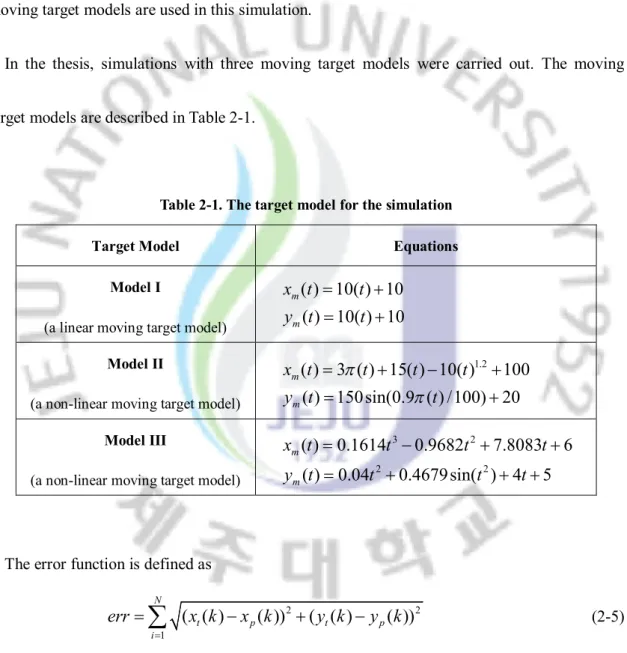
In the thesis, simulations with three moving target models were carried out. The moving target models are described in Table 2-1.

Table 2-1. The target model for the simulation

Target Model Equations

Model I

(a linear moving target model)

( ) 10( ) 10

m m

x t

t

y t

t

=

+

=

+

Model II

(a non-linear moving target model)

1.2 ( ) 3 ( ) 15( ) 10( ) 100 ( ) 150sin(0.9 ( ) /100) 20 m m x t t t t y t t

p

= + - + = + Model III

(a non-linear moving target model)

3 2 2 2 ( ) 0.1614 0.9682 7.8083 6 ( ) 0.04 0.4679sin( ) 4 5 m m x t t t t y t t t t = - + + = + + +

The error function is defined as

2 2 1

( ( )

( ))

( ( )

( ))

N t p t p i

err

x k

y k

=

å

-

+

-

(2-5) where x k y k_t( ), _t( ) are the x y, coordinates of the target’s true position, x k y k_p( ), _p( ) are the x y, coordinates of the target’s predicted position.

(18)

Example I: Tracking a linear moving target model (Model I) using the α-β tracker

The α-β tracker is operated for the four different values of the coefficient α, 0.3, 0.7, 1 and the variable obtained from (2-3). In the simulation, Gaussian noise with a mean of zero that is distributed with a variance of 0.1 is used. The coefficient β is obtained from (2-4). Figure 2-1 illustrates the tracking when a target has a straight trajectory with constant velocity.

-500 0 500 1000 1500 2000 2500 -500 0 500 1000 1500 2000 2500 Distance (m) D is ta n ce ( m )

The true data The measured data By the a-b tracker -500 0 500 1000 1500 2000 2500 -500 0 500 1000 1500 2000 2500 Distance (m) D is ta n ce ( m )

The true data The measured data By the a-b tracker

α= variable α= 0.3

α= 0.7 α= 1

Figure 2-1. Attained simulation results of the α-β tracker

(19)

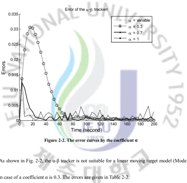
target model (Model I). Using (2-5), the errors are calculated for the four different values of the coefficient α, 0.3, 0.7, 1 and the variable from (2-3). Fig. 2-2 illustrate the error curves by the coefficient α. 0 20 40 60 80 100 120 140 160 180 200 0 0.005 0.01 0.015 0.02 0.025 0.03 0.035 Time (second) E rr o rs

Error of the a-b trackerr

a = variable

a = 0.3

a = 0.7

a = 1

Figure 2-2. The error curves by the coefficient α

As shown in Fig. 2-2, the α-β tracker is not suitable for a linear moving target model (Model I) in case of a coefficient α is 0.3. The errors are given in Table 2-2.

Table 2-2. Error of the α-β tracker

α variable 0.3 0.7 1

Error 112.2 1194.7 310.6 346.6

(20)

is a variable. However, the coefficient α 0.3 is not suitable in case of the linear moving target model (Model I).

Example II: Tracking a non-linear moving target model (Model II) using the α-β tracker

The α-β tracker is operated for the four different values of the coefficient α, 0.3, 0.7, 1 and the variable obtained from (2-3). In the simulation, the Gaussian noise used is same as in Example I. The coefficient β is obtained from (2-4). Fig. 2-3 illustrates the tracking when a target has a sharp turn trajectory with variable velocity.

-100 -50 0 50 100 150 200 -400 -300 -200 -100 0 100 200 Distance (m) D is ta n ce ( m )

The true data The measured data By the a-b tracker -100 -50 0 50 100 150 200 -150 -100 -50 0 50 100 150 Distance (m) D is ta n ce ( m )

The true data The measured data By the a-b tracker -100 -50 0 50 100 150 -150 -100 -50 0 50 100 150 Distance (m) D is ta n ce ( m )

The true data The measured data By the a-b tracker -100 -50 0 50 100 150 -250 -200 -150 -100 -50 0 50 100 150 Distance (m) D is ta n ce ( m )

The true data The measured data By the a-b tracker

α= variable α= 0.3

α= 0.7 α= 1

(21)

Fig. 2-3 shows the effect of varying the coefficient α. From the Fig. 2-3, the α-β tracker shows the best tracking performance when the coefficient α is a variable in case of the non-linear moving target model (Model II). However, the α-β tracker lost a target when the coefficient α is a variable. Using (2-5), the errors are calculated for the four different values of the coefficient α, 0.3, 0.7, 1 and the variable from (2-3). The error curves by the coefficient α are as shown in Fig. 2-4. 0 20 40 60 80 100 120 140 160 180 200 0 50 100 150 200 250 300 350

Error of the a-b trackerr

Time (second) D is ta n ce ( m ) a = variable a = 0.3 a = 0.7 a = 1

Figure 2-4. The error curves by the coefficient α

(22)

the coefficient α is a variable. The errors are given in Table 2-3.

Table 2-3. Error of the α-β tracker

α variable 0.3 0.7 1

Error 3560.9 1178.5 397.0 497.7

From the table 2-3, a variable coefficient is not suitable in case of the non-linear moving target model (Model II). And when coefficient α is 0.7, the α-β tracker gives the best tracking performance.

(23)

2.2.2 The Kalman Tracker

The state equation of a target is given by [16]

1

k k k

X

₊

=

FX

+

W

(2-6)

where

X

_k

=

[

x

_k

y

_k

x

&

_k

y

&

_k

]

is state vector at time k.

x

_k,

y

_k and

x&

_k,

y&

_k represent the positions and speeds in

x

, ycoordinates, respectively.

The transition matrix F is given by

1 0

0 0 1 0

0 0 0 1

T

F

é

ù

ê

ú

ê

ú

=

ê

ú

ê

ú

ë

û

(2-7)

where T is the sampling interval and

W

_k is the process noise vector with covariance

matrix

Q

.

The measurement equation is

( )

k k k

z k

=

HX

+

V

(2-8)

where

V

_k is the measurement noise vector with covariance matrix R which is assumed to be

white with zero mean, and no correlation exists with

W

_k

The measurement matrix H is given by

1 0 0 0

0 1 0 0

H

_{= ê}

é

ù

_ú

ë

û

(2-9)

(24)

1 1 1 1 1

ˆ

_k

ˆ

_k T k k k

x

Fx

P

FP F

Q

- -- -

-=

=

+

(2-10)

where

P

_k_-₁ is estimation error covariance matrix.

The filtered estimate measurement update equations are

1 1 1 1 1 1 ˆ ˆ ( ˆ ) Re k k k k k T k k k k k x x K z Hx P P P H HP - -- - -= + -= - (2-11) where the Kalman gain matrix is defined as

1 1 1 Re (Re) T k k T k k HP H R K P H -= + = (2-12) and estimation error covariance is given by

1

(

)

k k k k

P

= -

I K H P

_- (2-13)

The Kalman tracking algorithm can be denoted as follows:

Procedure {Design Algorithm of the Kalman tracker}

Generate the measured position

z N

( )

Set the number of iteration of the Kalman tracker N; Set the initial state vector

ˆx

₀;

Set the measurement noise covariance R and the process noise covariance P, Q; Set the transition matrix F and the measurement matrix H;

For k=1, 2, …, N

Extrapolate the most recent state estimate to the present time; Compute the Kalman gain;

(25)

Update the state estimate;

Compute the covariance of the estimation error

End

Example III:Tracking a linear moving target model (Model I) using the Kalman tracker

The Kalman tracker is operated for the four different values of the noise variance Q, 1, 0.1, 0.01 and 0.001. In the simulation, the Gaussian noise used is same as in Example I. Fig. 2-5 illustrates the tracking when a target has a sharp turn trajectory with constant velocity.

0 500 1000 1500 2000 2500 0 500 1000 1500 2000 2500 Distance (m) D is ta n ce ( m )

The true data The measured data By the Kalman tracker

-500 0 500 1000 1500 2000 -500 0 500 1000 1500 2000 Distance (m) D is ta n ce ( m )

Q = 1 Q = 0.1

Q = 0.01 Q = 0.001

Figure 2-5. Attained simulation results of the Kalman tracker

(26)

target model (Model I). Using (2-5), the errors are calculated for the four different values of the noise covariance Q, 1, 0.1, 0.01 and 0.001. The error curves by the noise covariance Q are as shown in Fig. 2-6. 0 20 40 60 80 100 120 140 160 180 200 0 5 10 15 20 25 30 35 40 45

50 Error of the Kalman tracker

Time (second)

D

is

ta

n

ce

(

m

)

Q = 1 Q = 0.1 Q = 0.01 Q = 0.001

Figure 2-6. The error curves by the noise covariance

As shown in Fig. 2-6, the Kalman tracker shows the best tracking performance when the noise variance Q is 1, in case of the linear moving target model (Model I).

Table 2-4, Error of the Kalman tracker

Q 1 0.1 0.01 0.001

(27)

From the table 2-4, as the noise covariance Q decreases, the error of the Kalman tracker tends to increase.

Example IV: Tracking a non-linear moving target model (Model II) using the Kalman tracker

The Kalman tracker is operated for the four different values of the noise variance Q, 1, 0.1, 0.01 and 0.001. In the simulation, the Gaussian noise used is same as in Example I. Fig. 2-7 illustrates the tracking when a target has a sharp turn trajectory with variable velocity.

-100 -50 0 50 100 150 200 -150 -100 -50 0 50 100 150 Distance (m) D is ta n ce ( m )

-100 -50 0 50 100 150 -100 -50 0 50 100 150 Distance (m) D is ta n ce ( m )

-100 -50 0 50 100 150 -150 -100 -50 0 50 100 150 Distance (m) D is ta n ce ( m )

Q = 1 Q = 0.1

Q = 0.01 Q = 0.001

Figure 2-7. Attained simulation results of the Kalman tracker

(28)

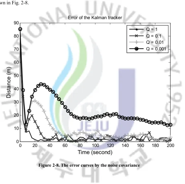
covariance Q is 1. However, the Kalman tracker lost a target when the noise covariances Q are 0.1, 0.01 and 0.001. Using (2-5), the errors are calculated for the four different values of the noise covariance Q, 1, 0.1, 0.01 and 0.001. The error curves by the noise covariance Q are as shown in Fig. 2-8. 0 20 40 60 80 100 120 140 160 180 200 0 10 20 30 40 50 60 70 80 90

Error of the Kalman tracker

Time (second)

D

is

ta

nc

e

(m

)

Q = 1 Q = 0.1 Q = 0.01 Q = 0.001

Figure 2-8. The error curves by the noise covariance

As shown in Fig. 2-8, the Kalman tracker shows the best tracking performance when the noise variance Q is 1 in case of the linear moving target model (Model I). The errors are given in Table 2-5.

(29)

Table 2-5. Error of the Kalman tracker

Q 1 0.1 0.01 0.001

Error 225.9 338.8 627.1 1338.3

From the table 2-5, the Kalman tracker shows the best tracking performance when the noise covariance Q is 1. However, the Kalman tracker lost a target in case of noise covariance Q is 0.001 for a non-linear moving target model (Model II).

(30)

2.3 Proposed Algorithm

2.3.1 The Switched Slide Window Tracker

The switched slide window tracker (SSWT) is composed of the α-β tracker to find the initial parameters and slide window tracker (SWT) to track the targets. Fig. 2-9 shows the flow chart of the proposed SSWT. First of all, the α-β tracker is running until the initial parameters for a particular window size are obtained. Then the slide window tracker predicts the next position using the weight value and the previously estimated position.

SELECT THE WINDOW SIZE

WINDOW SIZE > INITIAL PARAMETERS ? SLIDE WINDOW TRACKER: CALCULATE PREDICTED POSITION

START

NO α-β TRACKER:

CALCULATE PREDICTED POSITION

YES

END

NO NUMBER OF DATA < ITERATION ?

YES

SELECT THE WINDOW SIZE

WINDOW SIZE > INITIAL PARAMETERS ? SLIDE WINDOW TRACKER: CALCULATE PREDICTED POSITION

START

NO α-β TRACKER:

CALCULATE PREDICTED POSITION

YES

END

NO NUMBER OF DATA < ITERATION ?

YES

Figure 2-9. Flow chart for the SSWT

(31)

The SSWT is designed exploiting a piecewise linear model for a moving target. If a piecewise linear model is used during the short time of a trajectory, the non-linear model can be treated as a linear model as shown in Fig. 2-10.

Piecewise linear model

Time

D

is

ta

n

c

e

)

2 (

k

-x

_F

)

3 (

k

-x

_F

)

1 (

k

-x

_F

x

F

(k

)

Piecewise linear model

Time

D

is

ta

n

c

e

)

2 (

k

-x

_F

)

3 (

k

-x

_F

)

1 (

k

-x

_F

x

F

(k

)

Figure 2-10. A piecewise linear model for non-linear moving target

Using the piecewise linear model, assume that our trajectory is satisfied as piecewise linear moving at the same interval. The target position could be predicted by the present estimated position. If the target position varies linearly, the predicted target position can be expressed by the linear combination of the previously estimated position [7].

When initial positions are obtained greater than the window size, the process is switched to SWT from the α-β tracker. The SWT can be defined by following equations:

(32)

1

( )

[ ( )

( )],

(

1)

(

)

[ (

1)

(

)],

F p m p M p F m F F m

X k

x k

x k M

x k m

x k M

m

w

=

+

-+ =

-

+

å

- + -

-

(2-14)

where x k_m( ) is the

x

coordinate of the target’s measured position, x kp( +1) is the

x

coordinate of the target’s predicted position,

x k

_F

( )

is the

x

coordinate of the filtered target

position,

w

_m is the weight value [10], and

m

is the coefficient for the measurement update of the slide window tracker (In the thesis,

m a

= .). From (2-14), we can easily extend the equation for a 2-D problem.

In the thesis, weight values

w

_m are obtained for window size M=2, 3, 4 and 5 and the results are shown in Table 2-6.

Table 2-6. The weight values Window size Weight value 1

w

₂

w

₃

w

₄

w

₅ 2 -1 2 3 -2/3 1/3 4/3 4 -0.5 0 0.5 1 5 -0.35 -0.2 0.25 0.5 0.8

Computer simulation was done to prove the performance of the proposed algorithm. The proposed algorithm as described in Fig. 2-9 can be denoted as follows:

(33)

Procedure {Design Algorithm of the SSWT}

Generate the measured position

x N

_m

( )

; Choose a window size M (

M

=

2,3,4,5

);

Set the number of iteration of the α-β tracker MM (MM =M +1; Set the initial position and velocity for α-β tracker;

Select the α-β coefficients;

For k=1, 2, …, MM

Compute initial positions using the α-β tracker in (2-1);

End

For k=MM+1, MM+2, …, N

Switch to SWT;

Compute the predicted positions using (2-14);

End

For an α-β tracker, the criterion for selecting the α-β coefficients is based on the best linear track fitted to radar data in a least squares sense. The α-β coefficients is given by [4]

))

1 (

/(

))

1

2 (

-

+

=

k

a

. (2-15)

))

1 (

/(

6 +

=

k

b

. (2-16)

where k is the number of the scan or target observation (k>2).

In the simulation, the radar measures the positions of the moving target once per second, and 200 iterations was performed. The window size for the SWT is M=2, 3, 4, 5. Two target models, a linear moving target model and a non-linear moving target models are used to verify the

(34)

proposed algorithm.

Example V: Tracking a non-linear moving target model (Model I) using the SSWT

The SSWT is operated for the four different values of the window size M, 2, 3, 4 and 5. In the simulation, the Gaussian noise used is same as in Example I. Fig. 2-11 illustrates the tracking when a target has a straight trajectory with constant velocity.

-500 0 500 1000 1500 2000 2500 -500 0 500 1000 1500 2000 2500 Distance (m) D is ta nc e (m )

The true data The measured data By the SSWT -500 0 500 1000 1500 2000 -500 0 500 1000 1500 2000 Distance (m) D is ta nc e (m )

The true data The measured data By the SSWT -500 0 500 1000 1500 2000 2500 -500 0 500 1000 1500 2000 2500 Distance (m) D is ta nc e (m )

The true data The measured data By the SSWT

M = 2 M = 3

M = 4 M = 5

Figure 2-11. Attained simulation results of the SSWT

As shown in Fig. 2-11, the SSWT shows good tracking performance for a linear moving target model (Model I). Using (2-5), the errors are calculated for the four different values of the window size M, 2, 3, 4 and 5. The error curves by the window size M are as shown in Fig. 2-12.

(35)

0 20 40 60 80 100 120 140 160 180 200 0 10 20 30 40 50 60 70

Error of the switched slide window tracker

Time (second) D is ta n ce ( m ) M = 2 M = 3 M = 4 M = 5

Figure 2-12. The error curves by the window size.

As shown in Fig. 2-12, the SSWT shows good tracking performance for a linear moving target model (Model I). The errors are given in Table 2-7.

Table 2-7. Error of the switched slide window tracker

M 2 3 4 5

Error 187.5 138.7 154.1 129.7

From the table 2-7, a small window size gives a better tracking performance for a linear moving target model (Model I).

(36)

The SSWT is operated for the four different values of the window size M, 2, 3, 4 and 5. In the simulation, the Gaussian noise used is same as in Example I. Fig. 2-13 illustrates the tracking when a target has a sharp turn trajectory.

-100 -50 0 50 100 150 -400 -300 -200 -100 0 100 200 Distance (m) D is ta n ce ( m )

The true data The measured data By the SSWT -100 -50 0 50 100 150 -400 -300 -200 -100 0 100 200 Distance (m) D is ta n ce ( m )

The true data The measured data By the SSWT -100 -50 0 50 100 150 -500 -400 -300 -200 -100 0 100 200 Distance (m) D is ta n ce ( m )

The true data The measured data By the SSWT

M = 2 M = 3

M = 4 M = 5

Figure 2-13. Attained simulation results of the SSWT

As shown in Fig.2-13, the SSWT shows the best tracking performance when the window size

M is 2. Using (2-5), the errors are calculated for the four different values of the window size M,

(37)

0 20 40 60 80 100 120 140 160 180 200 100

101 102 103

Error of the switched slide window tracker

Time (second) D is ta nc e (m ) M = 2 M = 3 M = 4 M = 5

Figure 2-14. The error curves by the window size.

From the table 2-8, the SSWT shows the best tracking performance when the window size M is 2, in case of a non-linear moving target model (Model II).

Table 2-8. Error of each tracking algorithm

M 2 3 4 5

Error 677.5 816.9 1072.3 1306.7

From the results, the SSWT shows better tracking performance when the window size M is small in case of a non-linear moving target. The errors are given in Table 2-8.

(38)

2.3.2 Comparison of Each Algorithm

In this simulation, the target model II and III are used for comparison. In the simulation, the Gaussian noise used is same as in Example I.

Fig. 2-15 illustrates the tracking results by changing the coefficient α of the α-β tracker for a non-linear moving target model (Model II). The coefficient β is obtained from (2-4). The noise covariance Q of the Kalman tracker and window size M of the SSWT are set as 1 and 2, respectively. -100 -50 0 50 100 150 200 -500 -400 -300 -200 -100 0 100 200 Distance (m) D is ta n ce ( m )

The true data By the SSWT By the a-b tracker By the Kalman tracker

-100 -50 0 50 100 150 -500 -400 -300 -200 -100 0 100 200 Distance (m) D is ta n ce ( m )

-100 -50 0 50 100 150 -400 -300 -200 -100 0 100 200 Distance (m) D is ta n ce ( m )

α= variable Q = 1 M = 2 α= 0.3 Q = 1 M = 2 α= 1 Q = 1 M = 2 α= 0.7 Q = 1 M = 2 (a) (b) (c) (d)

(39)

As shown in Fig. 2-15, the Kalman tracker and the SSWT give good tracking performance for a non-linear moving target model (Model II). To compare the tracking performance of each algorithm, the errors are calculated using (2-5). The error curves of each tracking algorithm are as shown in Fig. 2-16. 0 20 40 60 80 100 120 140 160 180 200 0 50 100 150 200 250 300 350 Time (second) D is ta n ce ( m )

Error of the switched slide window tracker Error of the a-b tracker

0 20 40 60 80 100 120 140 160 180 200 0 50 100 150 200 250 300 350 Time (second) D is ta n ce ( m )

0 20 40 60 80 100 120 140 160 180 200 0 50 100 150 200 250 300 Time (second) D is ta n ce ( m )

Figure 2-16. The error curves of each algorithm

As shown in Fig. 2-16, the α-β tracker gives the worst tracking result when the coefficient α is a variable. The errors of each algorithm are given in Table 2-9.

(40)

Table 2-9. Error of each tracking algorithm Error Type of algorithm (a) (b) (c) (d) The SSWT 629.2 653.1 728.2 723.3 The α-β tracker 3486.4 1152.8 426.7 525.4

The Kalman tracker 196.7 204.1 224.8 221.2

From the table 2-9, the Kalman tracker gives the best tracking performance in case of a non-linear moving target model (Model II).

Fig. 2-17 illustrates the tracking results by changing the noise covariance Q of the Kalman tracker for a non-linear moving target model (Model II). The coefficient β is obtained from (2-4). The coefficient α of the α-β tracker and window size M of the SSWT are set as the variable obtained from (2-3) and 2, respectively.

(41)

-100 -50 0 50 100 150 200 -500 -400 -300 -200 -100 0 100 200 Distance (m) D is ta n ce ( m )

α= variable Q = 1 M = 2 α= variable Q = 0.1 M = 2 α= variable Q = 0.001 M = 2 α= variable Q = 0.01 M = 2 (a) (b) (c) (d)

Figure 2-17. The trajectory of each algorithm

As shown in Fig. 2-17, the SSWT gives good tracking performance for a non-linear moving target model (Model II). To compare the tracking performance of each algorithm, the errors are calculated using (2-5). The error curves of each tracking algorithm are as shown in Fig. 2-18.

(42)

As shown in Fig. 2-18, the α-β tracker gives the worst tracking result. The errors of each algorithm are given in Table 2-10.

Table 2-10. Error of each tracking algorithm Error Type of algorithm

(a) (b) (c) (d)

The SSWT 691.6 674.7 699.4 668.9

The α-β tracker 3558.9 3537.1 3547.8 3561.1

From the table 2-10, the Kalman tracker and the SSWT give the good tracking performance in case of a non-linear moving target model (Model II).

(43)

Fig. 2-19 illustrates the tracking results by changing the window size M of the SSWT for a non-linear moving target model (Model II). The noise covariance Q of the Kalman tracker and the coefficient α of the α-β tracker are set as 1 and the variable obtained from (2-3), respectively. The coefficient β is obtained from (2-4).

α= variable Q = 1 M = 2 α= variable Q = 1 M = 3 α= variable Q = 1 M = 5 α= variable Q = 1 M = 4 (a) (b) (c) (d)

As shown in Fig. 2-19, the Kalman tracker and the SSWT give good tracking performance for a non-linear moving target model (Model II). To compare the tracking performance of each algorithm, the errors are calculated using (2-5). The error curves of each tracking algorithm are

(44)

as shown in Fig. 2-20. 0 20 40 60 80 100 120 140 160 180 200 0 50 100 150 200 250 300 Time (second) D is ta n ce (m )

0 20 40 60 80 100 120 140 160 180 200 0 50 100 150 200 250 300 Time (second) D is ta n ce (m )

0 20 40 60 80 100 120 140 160 180 200 0 50 100 150 200 250 300 350 Time (second) D is ta n ce (m )

0 20 40 60 80 100 120 140 160 180 200 0 50 100 150 200 250 300 Time (second) D is ta n ce (m )

(a) (b) (c) (d)

The SSWT 679.0 878.5 1076.0 1345.5

The α-β tracker 3558.9 3570.0 3582.8 3558.3

(45)

From the table 2-11, the Kalman tracker and the SSWT give good tracking performance in case of a non-linear moving target model (Model II).

Fig. 2-21 illustrates the tracking results by changing the coefficient α of the α-β tracker for a non-linear moving target model (Model III). The coefficient β is obtained from (2-4). The noise covariance Q of the Kalman tracker and window size M of the SSWT are set as 1 and 2, respectively. 0 2 4 6 8 10 12 14 x 105 0 500 1000 1500 2000 2500 Distance (m) D is ta n ce ( m )

0 2 4 6 8 10 12 14 x 105 0 500 1000 1500 2000 2500 Distance (m) D is ta n ce ( m )

(46)

a non-linear moving target model (Model III). To compare the tracking performance of each algorithm, the errors are calculated using (2-5). The error curves of each tracking algorithm are as shown in Fig. 2-22. 0 20 40 60 80 100 120 140 160 180 200 0 0.5 1 1.5 2 2.5 3 3.5 4 4.5x 10 5 Time (second) D is ta n ce (m )

0 20 40 60 80 100 120 140 160 180 200 0 1 2 3 4 5 6x 10 4 Time (second) D is ta n ce (m )

0 20 40 60 80 100 120 140 160 180 200 0 0.5 1 1.5 2 2.5 3 3.5 4x 10 4 Time (second) D is ta n ce (m )

As shown in Fig. 2-22, the Kalman tracker gives the best tracking result. The errors of each algorithm are given in Table 2-12.

(47)

Table 2-12. Error of each tracking algorithm Error Type of algorithm (a) (b) (c) (d) The SSWT 671710 671720 671730 671730 The α-β tracker 5275300 1151000 190640 74448

The Kalman tracker 24833 24837 24840 24837

From the table 2-12, the Kalman tracker gives the best tracking performance in case of a non-linear moving target model (Model III).

Fig. 2-23 illustrates the tracking results by changing the noise covariance Q of the Kalman tracker for a non-linear moving target model (Model III). The coefficient α of the α-β tracker and window size M of the SSWT are set as the variable obtained from (2-3) and 2, respectively. The coefficient β is obtained from (2-4).

(48)

As shown in Fig. 2-23, the Kalman tracker and the SSWT give good tracking performance for a non-linear moving target model (Model III). To compare the tracking performance of each algorithm, the errors are calculated using (2-5). The error curves of each tracking algorithm are as shown in Fig. 2-24.

(49)

0 20 40 60 80 100 120 140 160 180 200 0 0.5 1 1.5 2 2.5 3 3.5 4 4.5x 10 Time (second) D is ta n ce ( m )

0 20 40 60 80 100 120 140 160 180 200 0 0.5 1 1.5 2 2.5 3 3.5 4 4.5x 10 5 Time (second) D is ta n ce ( m )

(a) (b) (c) (d)

The SSWT 671710 671710 671730 671710

The α-β tracker 5275200 5275200 5275200 5275200

(50)

non-linear moving target model (Model III).

Fig. 2-25 illustrates the tracking results by changing the window size M of the SSWT for a non-linear moving target model (Model III). The noise covariance Q of the Kalman tracker and the coefficient α of the α-β tracker are set as 1 and the variable obtained from (2-3), respectively. The coefficient β is obtained from (2-4).

As shown in Fig. 2-25, the Kalman tracker and the SSWT give good tracking performance for a non-linear moving target model (Model III). To compare the tracking performance of each

(51)

algorithm, the errors are calculated using (2-5). The error curves of each tracking algorithm are as shown in Fig. 2-26. 0 20 40 60 80 100 120 140 160 180 200 0 0.5 1 1.5 2 2.5 3 3.5 4 4.5x 10 5 Time (second) D is ta n ce (m )

0 20 40 60 80 100 120 140 160 180 200 0 0.5 1 1.5 2 2.5 3 3.5 4 4.5x 10 5 Time (second) D is ta n ce (m )

Table 2-14. Error of the each tracking algorithm Error

Type of algorithm

(a) (b) (c) (d)

The SSWT 671700 1093200 1595800 2139400

(52)

From the table 2-14, the Kalman tracker gives the best tracking performance in case of a non-linear moving target model (Model III).

From all the results, on an average, the SSWT shows a good performance for not only a linear moving target model but also a non-linear moving target model. As shown in the all figures, the proposed method has better performance than the α-β tracker.

(53)

2.4 Implemented Simulator

The maritime radar simulator is made up of a DSP and a host PC. Fig. 2-27 illustrates the functional block diagram of the maritime radar simulator system.

GUI software

Calculate

Initialization

The switched slide window tracker The Kalman tracker

The α-β tracker

Generate ideal data

DSP BOARD

PC

Add noise Sta rt c_om m an_d Pred icte d posit ion & ve locit y RS-232 Display

Figure 2-27. Block diagram of simulator

A TMS320C6711 DSP board was used to implement the maritime radar simulator for proposed tracking algorithm. The photograph of the DSP is shown in Fig. 2-28.

(54)

A brief overview of the DSP board is shown in table 2-15.

Table 2-15. Specifications of the DSP board

DSP chip TI TMS320C6711

Type Floating Point DSP

Clock 200 MHz

ROM 1M Byte Flash Memory

Memory (SDRAM) 32M Byte

Internal Memory 64K Byte On-chip SRAM

EMIF 16-bit External Memory Interface

Serial Port 2 McBSP, User RS232, JTAG Port

Boot Mode ROM Boot

Power 5V

Power Consumption 3.5 Watt

The DSP board has an SRAM that can be used to store programs and data. The instruction rate of the chip is 235 MIPS [17]. The DSP board performs the operations such as generation of actual data and tracking of maneuvering target. The DSP board is programmed so as to allow the user to select a tracking algorithm from the α-β tracker, the Kalman tracker and the SSWT. The DSP board tracks the predicted position and velocity using the selected tracking algorithm and data association. The data association is to get the firm track. If the host PC sends the predicted target of a track to the DSP board, the DSP chip sets a rough validation gate around the targets. If there are detects in the rough validation gate, the validated detects are sent back to the host PC. Then, PC sets a more refined validation gate on them, and chooses the best detect

(55)

which will be used for the measurement update. The GUI software as shown in Fig. 2-29 is written by using LabVIEW 8.5.

Figure 2-29. The maritime radar simulator

Using the obtained position and velocity from the DSP, the GUI in a host PC displays the information of the moving targets as follows [18]:

(1) Filtered range and bearing to the target, (2) Predicted target range to the closest, (3) True course and speed of the target.

(56)

(57)

2.5 Conclusion

The SSWT to track moving targets was proposed in this research. The proposed algorithm can effectively track the target by using a piecewise linear model in a non-linear moving target trajectory.

To verify the proposed algorithm, the maritime radar simulator with the SSWT is implemented using a TMS320C6711 digital signal processor (DSP) board and LabVIEW 8.5 and is compared against the α-β tracker and the Kalman tracker.

The proposed algorithm is more effective than the α-β tracker for non-linear moving targets. The computation time for each tracking algorithm running on this board was estimated. It turned out that our algorithm requires much less time than the Kalman tracking algorithm. The proposed tracking algorithm has a couple of advantages over the Kalman tracking algorithm in terms of computation time, and non-requirement of the statistical characteristics of a target.

Our implementation by utilizing the proposed algorithm can improve the tracking performance of the maritime radar.

(58)

CHAPTER 3 The Parametric Array Sonar System

3.1 Introduction

The sonar system has an important role in underwater communication. In the underwater communications, transmitted acoustic signal is corrupted by interference from multipath [10]. A parametric array transducer is capable of radiating a narrow beam with very low sidelobe levels [11]. In certain cases, the parametric array transducer can help the multipath problem. To improve the performance of the underwater communications, the statistical signal processing methods will be required.

In the thesis, the sonar communication system using a parametric array transducer was demonstrated. The on-off keying scheme was applied to modulate the signal [19]. For a good communication, the maximum likelihood method using averaged signal for a particular window size is used in the system [12].

The system is composed of a parametric array transducer, a NI PXI system, a microphone, a power amplifier, a PC with DAQCard, and the control software developed by LabVIEW 8.5. The sonar communication system has GUI which allows the user to change the parameter. The GUI can also be easily modified based on the characteristics of a parametric array transducer. The implemented system can effectively evaluate the performance of the parametric array

(59)

transducer.

Section 3.2 gives a brief overview of the detection algorithm. Section 3.3 presents the implemented transmitter, receiver and the experimental results. Finally, Section 3.4 describes some of the research results.

(60)

3.2 Maximum Likelihood Method

The decision rule defined as [12]

(

) (

)

(

) (

)

1 1 2 2 2 1 ( ) d if p z m z m d z d if p z m z m ì > ï = í > ïî (3-1) 1 2

:

m z n

m z s n

=

= +

(3-2)

where the observation of

m

₁ is the zero-mean unit-variance gaussian random noise, the

observation of

m

₂ is

s n

+

,

s

is the mean value.

The conditional probability density of z given

m

₁ or

m

₂ as

(

)

(

)

2 1 2 2

1 exp

2

1 (

)

exp

2

2 z

p z m

z s

p z m

p

-=

(3-3)

The decision regions are

(

) (

)

{

}

(

) (

)

{

}

1 1 1 2 1 1

:

Z

z p z m

p z m

Z

z p z m

p z m

=

>

=

<

(3-4)

The likelihood ratio L

( )

z defined as

( )

(

₍

2

₎

)

1

p z m

z

p z m

L

=

(3-5) Then

Z

₁ and

Z

₂ may be defined as

( )

{

}

( )

{

}

1 2

:

1 :

1 Z

z

Z

z

=

L

<

=

L

>

(3-6)

(61)

It can be expressed shortly

( )

2 1 1 d d z >_< L (3-7) Using above the equations, the problem can be solved

( )

(

₍

₎

)

(

)

(

)

(

)

(

)

(

)

2 2 2 1 2 2

1 2

exp

/ 2

1 2

exp

/ 2

exp

2

2 exp

2 z s

p z m

z

p z m

z

z s

z

z s

p

é

_{- -}

ù

ë

û

L

=

é

-

ù

ë

û

é

ù

-

_ë

-

_û

=

-=

(3-8)

The decision rule can be written as

2 1 (2 ) exp 1 2 d d z s > < (3-9)

Take the natural logarithm of (3-9)

2 1 0 2 2 d d z s > < (3-10) Then (3-11) is obtained 2 1 2 d s d z_<> (3-11)

and the decision regions can be defined as

1 2 2 2 2 2

:

,

:

,

s s s s

Z

z z

Z

z z

ì

ü æ

ö

=

_í

<

_{ý ç}

= -¥

_÷

î

þ è

ø

ì

ü æ

ö

=

_í

>

_{ý ç}

=

¥

_÷

î

þ è

ø

(3-12)

(62)

explained in section 3.3. 0.00 0.01 0.02 0.03 0.04 0.05 0.06 0.07 0.08 0.09 0.10 -0.25 -0.2 -0.15 -0.1 -0.05 0 0.05 0.1 0.15 0.2 0.25 Time [second] A m pl itu de [ vo lta ge ]

Figure 3-1. Measured signal

To detect the signal, averaging technique was applied, additionally. The averaged signal is obtained by 1 1 1 1 2 2 2 1 1 : 1 : N i i i N i i i m z s n N m z s n N = = = + = +

å

(3-13)

where N is the sample number.

(63)

0.01 0.02 0.03 0.04 0.05 0.06 0.07 0.08 0.09 0.10 0 0.02 0.04 0.06 0.08 0.1 0.12 0.14 0.16 Time [second] A m pl itu de [ vo lt ag e]

Figure 3-2. The average value of the signal

As shown in Fig. 3-2, the signal is absolute and averaged. Fig. 3-3 illustrates the probability density function of the averaged signal. The averaged value of the signal has Gaussian distribution. 0 0.05 0.1 0.15 0.2 0 0.2 0.4 0.6 0.8 1 Normalized signal P D F pdf of s1+n1 pdf of s2+n2 Decision

(64)

The decision rule from the ML method is

(

)

2 1 2 1 2 d d s s z_<> + (3-13)

where

s

₁ and

s

₂ are mean values.

The standard deviations of

s

₁

+

n

₁ and

s

₂

+

n

₂ are 0.0025 and 0.0169, respectively. The

means of

s

₁

+

n

₁ and

s

₂

+

n

₂ are 0.0094 and 0.1658, respectively. Hence, if z >0.0876, we

(65)

3.3 Implemented System

3.3.1 Transmitter

The parametric array sonar system consists mainly of transmitter and receiver. The block diagram of the transmitter is shown in Fig. 3-4 [20].

Data input

Controller (NI PXI-6070E)

Modulation

D/A

Parametric

Array

Transducer

Power

Amplifier

Figure 3-4. Block diagram of transmitter

The transmitter is composed of a parametric array transducer, a NI PXI system and a power amplifier. The PXI system plays a role in the modulation and the digital to analog conversion (DAC). The control software is programmed by LabVIEW 8.5. A brief overview of the NI PXI system is shown in Table 3-1.

Table 3-1. Specifications of PXI-6070E

Item Description

Output Resolution 12 bits

Output Rate 1 MS/s

Output Range ±10 V

FIFO Buffer Size 2,048 samples

(66)

transducers laboratory of Pohang University of Science and Technology [21]. Fig. 3-5 shows the structure of the prototype parametric array transducer.

Figure 3-5. Structure of the prototype parametric array transducer

The prototype parametric array transducer has 82 kHz and 122 kHz resonance frequencies, and its size is 50mm x 50mm.

Statistical Signal Processing Algorithms for Radar and Sonar System