Spatial assessment of soil contamination by heavy metals from informal electronic waste recycling in Agbogbloshie, Ghana

(1)

This is an Open Access article distributed under the terms of the Creative Commons Attribution Non-Commercial License (http://creativecommons.org/ licenses/by-nc/3.0/) which permits unrestricted non-commercial use, distribution, and reproduction in any medium, provided the original work is properly cited.

Page 1 of 10 http://e-eht.org/

Introduction

Changing electrical electronic equipment consumer’s lifestyle and the ever growing demand for newer and more efficient technologies are contributing to the increasing rate of obsolesce of electrical materials [1,2]. An estimated 41 million tons of electrical electronic equipment waste, also known as electronic waste (e-waste), were generated globally in 2014 [3]. Fifty to

eighty percent of electrical electronic equipment meant for dis-posal and recycling in developed countries are either legally or illegally shipped to developing countries under the disguise of slightly used or charity materials [4]. Some of these equipment end up in informal recycling sites where primitive recycling methods, such as the open burning of cables, fridge, and televi-sion casings, are performed, exposing the environment and en-tire communities to pollution [5]. Contamination of the

envi-Spatial assessment of soil contamination by heavy

metals from informal electronic waste recycling in

Agbogbloshie, Ghana

Vincent Nartey Kyere

1

_{, Klaus Greve}

2

_{, Sampson M. Atiemo}

3

1_{Center for Development Research (ZEF), University of Bonn, Bonn;}2_{Geography Institute, University of Bonn, Bonn,}

Germany; 3_{Ghana Atomic Energy Commission, Accra, Ghana}

• Original Article

http://dx.doi.org/10.5620/eht.e2016006

eISSN: 2233-6567

Objectives This study examined the spatial distribution and the extent of soil contami-nation by heavy metals resulting from primitive, unconventional informal electronic waste recycling in the Agbogbloshie e-waste processing site (AEPS) in Ghana.

Methods A total of 132 samples were collected at 100 m intervals, with a handheld glob-al position system used in taking the location data of the soil sample points. Observing all procedural and quality assurance measures, the samples were analyzed for barium (Ba), cadmium (Cd), cobalt (Co), chromium (Cr), copper (Cu), mercury (Hg), nickel (Ni), lead (Pb), and zinc (Zn), using X-ray fluorescence. Using environmental risk indi-ces of contamination factor and degree of contamination (Cdeg), we analyzed the

individ-ual contribution of each heavy metal contamination and the overall Cdeg. We further used

geostatistical techniques of spatial autocorrelation and variability to examine spatial dis-tribution and extent of heavy metal contamination.

Results Results from soil analysis showed that heavy metal concentrations were signifi-cantly higher than the Canadian Environmental Protection Agency and Dutch environ-mental standards. In an increasing order, Pb>Cd>Hg>Cu>Zn>Cr>Co>Ba>Ni con-tributed significantly to the overall Cdeg. Contamination was highest in the main working

areas of burning and dismantling sites, indicating the influence of recycling activities. Geostatistical analysis also revealed that heavy metal contamination spreads beyond the main working areas to residential, recreational, farming, and commercial areas.

Conclusions Our results show that the studied heavy metals are ubiquitous within AEPS and the significantly high concentration of these metals reflect the contamination factor and Cdeg, indicating soil contamination in AEPS with the nine heavy metals studied.

Keywords Electronic waste, Geostatistical techniques, Heavy metals, Contamination fac-tor, Degree of contamination

Correspondence: Vincent Nartey Kyere 3 Walter Flex Strasse, Bonn 53113, Germany Tel: +49-15218672980 Fax: +49-228731869 E-mail: [email protected] Received: January 22, 2016 Accepted: March 11, 2016 Published: March 17, 2016

(2)

http://e-eht.org/ Page 2 of 10

ronment due to uncontrolled e-waste recycling has been report-ed in Ghana and particularly Ghana’s largest e-waste recycling area Agbogbloshie [6-10]. The contamination of the environ-ment is driven by increased quantities of electrical e-waste in Ghana, which have created avenues and opportunities for indi-viduals to make a living by using unconventional, primitive, and crude recycling methods to recover precious and valuable met-als from e-waste. The uncontrolled recycling activities of indi-viduals, especially informal recyclers, and the absence of a well-structured management policy or strategy in Ghana have result-ed in pollution of the environment through the release of heavy metals from some of the unconventional recycling methods. This present study seeks to determine qualitatively and quanti-tatively heavy metal contamination from e-waste processing in Agbogbloshie, Ghana, and further through geostatistical tech-niques and spatial analysis to examine the spatial extent of heavy metal contamination from e-waste processing in Agbogbloshie. The results of this study can be useful in decision making pro-cesses for selecting appropriate remediation measures for con-taminated environments and protection of affected communi-ties from potential health hazards.

Materials and Methods

Study Area, Sample Collection, and Data Preparation

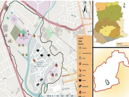
A total of 132 samples were collected from Agbogbloshie e-waste processing site (AEPS), using a 100 m interval grid based sampling procedure. AEPS is located close to the central busi-ness district of Ghana’s national capital (Figure S1) and consists of a number of clusters such as burning, dismantling, residential, recreational, commercial, worship, and school sites. Data collec-tion was conducted while observing all standard procedures to avoid cross contamination. The collected samples were air dried at room temperature, sieved through a 100 µm mesh, and pressed into pellets with a diameter of 2.5 cm using a 10-ton hy-draulic press. Heavy metal analysis was performed using an X-ray fluorescence (XRF) spectrometer, (at the Department of Geological Survey, Accra, Ghana), at a maximum power of 3000 W (60 Kv and 50 mA). The pelleted samples were placed on a disk which was put on the excitation source of the XRF for a 10-minute irradiation, using a silicon lithium Si (Li) detector with a resolution of 16 V with manganese and potassium alpha peaks throughout the procedure. To validate the procedure and ensure quality, International Atomic Energy Agency (IAEA) standard reference IAEA soil seven was irradiated five times and average values were compared with recommended values before analysis of prepared samples.

Statistical and Geostatistical Analysis

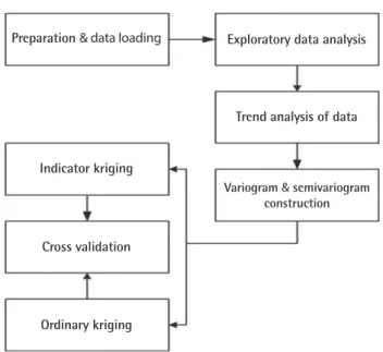
The study adopted the steps as shown in Figure S2 for the sta-tistical and geostasta-tistical analysis of the heavy metals barium (Ba), cadmium (Cd), cobalt (Co), chromium (Cr), copper (Cu), mercury (Hg), nickel (Ni), lead (Pb), and zinc (Zn) iden-tified in the soil samples. The selection of heavy metals used in our study was based on the criteria defined by the Dutch soil quality and guidance standards for contaminated lands and en-vironmental remediation [11].

Data Preparation and Exploratory Analysis

Heavy metal concentrations values together with the coordi-nates were listed in Microsoft Excel 2013 (Microsoft Co., Red-mond, WA, USA) and exploratory analysis of descriptive vari-ables, normality, and correlation between heavy metals were performed using R.3.2.1 software.

Trend Analysis and Variogram Construction

Trend analysis was performed using ArcGIS 10.1 to identify global trends or patterns which have to be taken into account before applying geostatistical interpolation. Variogram models and the global Moran’s index were used to examine spatial auto-correlation and spatial variability of heavy metals. Spatial vari-ability of the data was also assessed for each heavy metal using semivariogram or entropy voronoi maps before prediction or kriging of the data [12]. Exponential, spherical, and K-Bessel models were chosen as they obtained the best fit in the assess-ment of spatial autocorrelation for the heavy metal variables. The sill, nugget, and range for each of the models (exponential, K-Bessel and spherical) were also explored to ascertain variabili-ty and spatial dependency of the heavy metal dataset.

Kriging and Cross Validation

The final step in the geostatistical data analysis was kriging. With data not indicating any direction and no local drift or trend in the data set, anisotropic kriging, universal kriging, and co-kriging procedures were avoided in the prediction. The ordi-nary kriging process was performed on the degree of heavy met-al contamination.

Contamination Assessment

There are three categories of heavy metal assessment indices [13], which include (a) contamination indices [14] and metal enrichment index, (b) background enrichment indices [15]; in-dex of geoaccumulation [16], contamination factor (CF) and degree of contamination (Cdeg) [17], and (c) ecological risk

in-dices [18]. For the purpose and objectives of this study, the CF and Cdeg were chosen over the other indices for the following

(3)

http://e-eht.org/ Page 3 of 10 reasons:

CF and Cdeg indices overcome the requirement of using a

suit-able location for background concentration value by using con-tinental crust average as specified in [17].

The Cdeg complimented by the CF provides a comprehensive

picture of a particular site by aggregating individual heavy metal toxicity as single contamination index while pollution, metal en-richment, enrichment indices, and index of geoaccumulation are only suitable for evaluating single elements.

The CF and the Cdeg have been used over the years to assess or

ascertain the extent of heavy metal contamination of soils by comparing the results for the contaminants with different refer-ence or background levels [7,19–21]. The CF which evaluates environmental pollution by single substances is expressed as:

where is the CF of the element of interest; is the

con-centration of the element in the sample; is the background

concentration or the continental crustal average as was used by Muller [17]. The classification for contamination ranges from CF<1 as low CF; 1<CF≤3 as moderate CF; 3<CF≤6 as con-siderable CF and CF>6 very high CF. Complementing the CF is the Cdeg, which is the sum of CFs and describes the

contami-nation of the environment by all examined substances, further defining the quality of the environment. The Cdeg is expressed

as:

The Cdeg is useful to identify hot spots within the sampling

lo-cation. It is also categorized into four stages, such as Cdeg<8

im-plying a low, Cdeg 8≤Cdeg<16 indicating a moderate Cdeg, 16

≤Cdeg<32 indicating a considerable Cdeg, and Cdeg ≥32

indicat-ing a very high Cdeg.

Results

Descriptive Parameters of Heavy Metals Within Study

Area

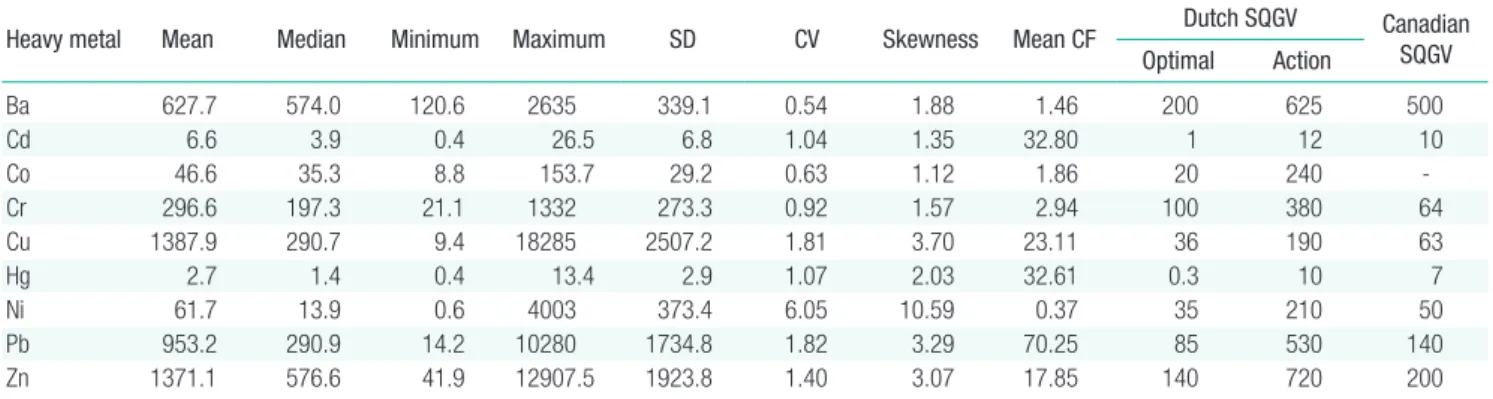
To evaluate the raw data set, we calculated the descriptive sta-tistics of mean, median, standard deviation, skewness, and coef-ficient of variation (CV) (Table 1). The concentrations of the heavy metals Ba, Cd, Co, Cr, Cu, Hg, Ni, Pb, and Zn under in-vestigation were extended over several orders of magnitudes. Compared with the Dutch and the Canadian Environmental Quality Standards for Soils, the mean values of Ba, Cu, Pb, and Zn were above both the optimal and action values of the Dutch and Canadian Soil Quality Guidance Values (SQGV) while those of Cd, Co, Hg, and Ni had mean values below action re-quired values of SQGV. The skewness values for Co, Cd, Cr, and Hg were relatively low, however, those for Ba, Pb, Zn, Cu, and Ni were high, indicating non-normality of the data set for these heavy metals. Further, CV values of Ni, Pb, Cu, and Zn were 6.05, 1.82, 1.81, and 1.40, respectively, and higher than those of Ba, Co, Cr, Cd, and Hg, suggesting that Ni, Pb, Cu, and Zn had greater variation among soils within the study area.

Table 1 also shows the mean CF for each of the heavy metals, indicating toxicity contribution. CFs of Ba, Co, Cr and Ni were within the moderate CFs while that of Cd, Cu, Hg, Pb and Zn were approximately 5, 4, 5, 11 and 3 times respectively within the high CF classification .

Correlation Between Heavy Metals

Table 2 shows the correlations between heavy metals. Our re-sults indicate significant correlation at p<0.05 of Ba with all heavy

metals apart from Ni and Pb. Cd also showed significant correla-tion at p<0.05 with all other heavy metals apart from Cr and Ni,

while Co showed significant correlation at p<0.05 with Cr, Cu,

Hg, and Zn, but weakly correlated with Ni and Pb. Table 2 shows

1

𝐶𝐶𝑓𝑓𝑖𝑖 =𝐶𝐶0−1

𝑖𝑖

𝐶𝐶𝑛𝑛𝑖𝑖 (1)

where 𝐶𝐶i𝑓𝑓 is the contamination factor of the element of interest; 𝐶𝐶i0−1is the concentration of the

element in the sample; 𝐶𝐶𝐶𝐶𝑛𝑛𝑛𝑛𝑖𝑖𝑖𝑖 is the background concentration or the continental crustal average

as was used by [17]. The classification for contamination ranges from CF < 1 as low CF; 1< CF ≤ 3 as moderate CF; 3< CF ≤ 6 as considerable CF and CF>6 very high CF. Complementing the contamination factor is the Cdeg, which is the sum of contamination factors and describes the contamination of the environment by all examined substances, further defining the quality of the environment. The Cdeg is expressed as:

𝐶𝐶deg =∑𝐶𝐶𝒊𝒊𝒇𝒇 (2)

The Cdeg is useful to identify hot spots within the sampling location. It is also categorized into

four stages, such as Cdeg< 8 implying a low Cdeg 8 ≤ Cdeg< 16 indicating a moderate Cdeg, 16 ≤

Cdeg< 32 indicating a considerable Cdeg, and Cdeg ≥ 32 indicating a very high Cdeg.

𝐶𝐶

𝑓𝑓𝑖𝑖

=

𝐶𝐶0−1

𝑖𝑖

where 𝐶𝐶

i𝑓𝑓

is the contamination factor of the element of interest; 𝐶𝐶

i0−1

is the concentration of the

element in the sample; 𝐶𝐶𝐶𝐶

𝑛𝑛𝑛𝑛𝑖𝑖𝑖𝑖

is the background concentration or the continental crustal average

as was used by [17]. The classification for contamination ranges from CF < 1 as low CF; 1< CF

≤ 3 as moderate CF; 3< CF ≤ 6 as considerable CF and CF>6 very high CF. Complementing the

contamination factor is the Cdeg, which is the sum of contamination factors and describes the

contamination of the environment by all examined substances, further defining the quality of the

environment. The Cdeg is expressed as:

𝐶𝐶

deg

=∑𝐶𝐶

𝒊𝒊𝒇𝒇 (2)

The Cdeg is useful to identify hot spots within the sampling location. It is also categorized into

four stages, such as C

deg

< 8 implying a low Cdeg 8 ≤ C

deg

< 16 indicating a moderate Cdeg, 16 ≤

C

deg

< 32 indicating a considerable Cdeg, and Cdeg ≥ 32 indicating a very high Cdeg.

𝐶𝐶

𝑓𝑓𝑖𝑖

=

𝐶𝐶0−1

𝑖𝑖

where 𝐶𝐶

i𝑓𝑓

is the contamination factor of the element of interest; 𝐶𝐶

i0−1

is the concentration of the

element in the sample; 𝐶𝐶𝐶𝐶

𝑛𝑛𝑛𝑛𝑖𝑖𝑖𝑖

is the background concentration or the continental crustal average

as was used by [17]. The classification for contamination ranges from CF < 1 as low CF; 1< CF

≤ 3 as moderate CF; 3< CF ≤ 6 as considerable CF and CF>6 very high CF. Complementing the

contamination factor is the Cdeg, which is the sum of contamination factors and describes the

contamination of the environment by all examined substances, further defining the quality of the

environment. The Cdeg is expressed as:

𝐶𝐶

deg

=∑𝐶𝐶

𝒊𝒊𝒇𝒇 (2)

The Cdeg is useful to identify hot spots within the sampling location. It is also categorized into

four stages, such as C

deg

< 8 implying a low Cdeg 8 ≤ C

deg

< 16 indicating a moderate Cdeg, 16 ≤

C

deg

< 32 indicating a considerable Cdeg, and Cdeg ≥ 32 indicating a very high Cdeg.

1

𝐶𝐶𝑓𝑓𝑖𝑖=𝐶𝐶0−1

𝑖𝑖

where 𝐶𝐶i𝑓𝑓 is the contamination factor of the element of interest; 𝐶𝐶i0−1is the concentration of the element in the sample; 𝐶𝐶𝐶𝐶𝑛𝑛𝑛𝑛𝑖𝑖𝑖𝑖 is the background concentration or the continental crustal average

The Cdeg is useful to identify hot spots within the sampling location. It is also categorized into four stages, such as Cdeg< 8 implying a low Cdeg 8 ≤ Cdeg< 16 indicating a moderate Cdeg, 16 ≤

1

𝑖𝑖

where 𝐶𝐶i𝑓𝑓 is the contamination factor of the element of interest; 𝐶𝐶i0−1is the concentration of the element in the sample; 𝐶𝐶𝐶𝐶𝑛𝑛𝑛𝑛𝑖𝑖𝑖𝑖 is the background concentration or the continental crustal average

The Cdeg is useful to identify hot spots within the sampling location. It is also categorized into four stages, such as Cdeg< 8 implying a low Cdeg 8 ≤ Cdeg< 16 indicating a moderate Cdeg, 16 ≤

1

𝑖𝑖

where 𝐶𝐶i𝑓𝑓 is the contamination factor of the element of interest; 𝐶𝐶i0−1is the concentration of the

element in the sample; 𝐶𝐶𝐶𝐶𝑛𝑛𝑛𝑛𝑖𝑖𝑖𝑖 is the background concentration or the continental crustal average

The Cdeg is useful to identify hot spots within the sampling location. It is also categorized into

four stages, such as Cdeg< 8 implying a low Cdeg 8 ≤ Cdeg< 16 indicating a moderate Cdeg, 16 ≤

Table 1. Summary statistics of heavy metal concentrations in soil

Heavy metal Mean Median Minimum Maximum SD CV Skewness Mean CF Dutch SQGV Canadian _SQGV Optimal Action Ba 627.7 574.0 120.6 2635 339.1 0.54 1.88 1.46 200 625 500 Cd 6.6 3.9 0.4 26.5 6.8 1.04 1.35 32.80 1 12 10 Co 46.6 35.3 8.8 153.7 29.2 0.63 1.12 1.86 20 240 -Cr 296.6 197.3 21.1 1332 273.3 0.92 1.57 2.94 100 380 64 Cu 1387.9 290.7 9.4 18285 2507.2 1.81 3.70 23.11 36 190 63 Hg 2.7 1.4 0.4 13.4 2.9 1.07 2.03 32.61 0.3 10 7 Ni 61.7 13.9 0.6 4003 373.4 6.05 10.59 0.37 35 210 50 Pb 953.2 290.9 14.2 10280 1734.8 1.82 3.29 70.25 85 530 140 Zn 1371.1 576.6 41.9 12907.5 1923.8 1.40 3.07 17.85 140 720 200 Concentration values are measured in ppm.

SD, standard deviation; CV, coefficient of variation; CF, contamination factor; SQGV, soil quality and guidance values; Ba, barium; Cd, cadmium; Co, cobalt; Cr, chromium; Cu, copper; Hg, mercury; Ni, nickel; Pb, lead; Zn, zinc.

(4)

that Ni only correlated significantly with Hg and weakly with all other heavy metals. The weak correlation of Cr and Ni with other heavy metals indicates sources of Cr and Ni independent of the other heavy metals, while the closely significant correla-tion between Ba, Cd, Co, Cu, Pb, and Zn indicates a source of similar origin or activity (such as Pb in printed circuit boards, Ba, Cd, Pb, Zn in cathode ray tube and batteries, Cu in cables and transformer coils, which are the main devices processed at AEPS).

Contamination Assessment

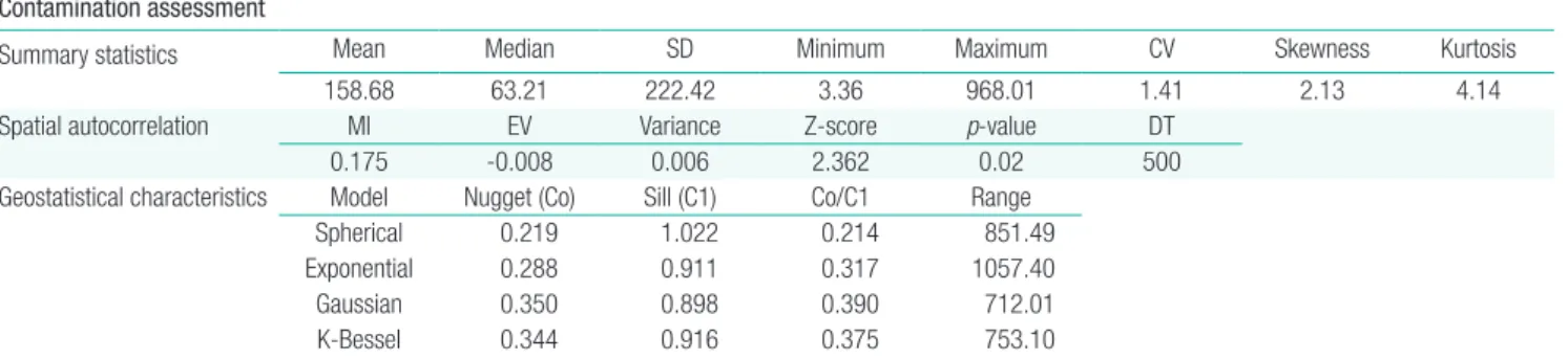
To describe the extent of contamination and to examine the toxicity of the metals under investigation, we calculated the Cdeg

as the sum of all CFs for each element present at a site or loca-tion. The mean Cdeg was 158.68, indicating a very high

contami-nation. The calculation of the Cdeg also revealed a 1.41 CV,

indi-cating high variability in the Cdeg, and a skewness value of 2.13,

showing a non-normal distribution and positively skewed data of the Cdeg (Table 3).

Geostatistical and Spatial Distribution of Degree of

Contamination

Geostatistical and spatial distribution assessment revealed spa-tial autocorrelation with a Moran’s index at a z-score of 2.362

and a p-value less than 0.05 (Table 3), indicating that the dataset

was spatially related and that both human induced and natural activities contributed to the high Cdeg.

Spatial Structure of Degree of Contamination

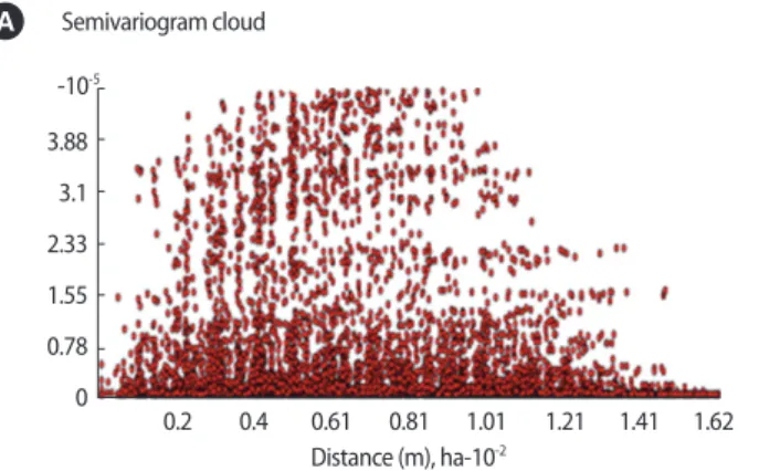
The spatial structure and spatial variation of the Cdeg were

fur-ther revealed by the variogram cloud (Figure S3A) and the en-tropy voronoi map (Figure S3B). The variogram cloud showed the best correlation in the northeast and southwest directions, indicating an omnidirectional orientation and thus isotropy in the Cdeg. Figure S3B shows the spatial variation in the Cdeg. Dark

and light green areas indicate little variation, while orange and dark red indicate greater variation. The map roughly indicates stationarity in the Cdeg.

Table 2. Correlation between heavy metal concentrations in soil at AEPS

Heavy metal Ba Cd Co Cr Cu Hg Ni Pb Zn Ba 1 Cd 0.712* 1 Co 0.748* 0.599* 1 Cr 0.604* 0.356 0.549* 1 Cu 0.449* 0.761* 0.435* 0.042 1 Hg 0.602* 0.804* 0.563* 0.190 0.855* 1 Ni 0.115 0.050 0.328 0.001 0.181 0.472* 1 Pb 0.341 0.724* 0.266 -0.139 0.903* 0.874* 0.250 1 Zn 0.549* 0.767* 0.598* 0.252 0.856* 0.778* 0.140 0.775* 1 AEPS, Agbogbloshie electronic waste processing site; Ba, barium; Cd, cadmium; Co, cobalt; Cr, chromium; Cu, copper; Hg, mercury; Ni, nickel; Pb, lead; Zn, zinc. *p<0.05. 1.628 1.357 1.085 0.814 0.543 0.271 0 _0.669_1.338_2.006_2.675_3.344_4.013_4.681 _5.35_6.019_{6.688 7.356} Averaged Binned Model Distance (m), ha-10-2

Figure 1. Isotropic semivariogam fitted with spherical model.

Table 3. Summary statistics and geostatistical parameters for degree of contamination

Contamination assessment

Summary statistics Mean Median SD Minimum Maximum CV Skewness Kurtosis 158.68 63.21 222.42 3.36 968.01 1.41 2.13 4.14 Spatial autocorrelation MI EV Variance Z-score p-value DT

0.175 -0.008 0.006 2.362 0.02 500 Geostatistical characteristics Model Nugget (Co) Sill (C1) Co/C1 Range

Spherical 0.219 1.022 0.214 851.49 Exponential 0.288 0.911 0.317 1057.40 Gaussian 0.350 0.898 0.390 712.01 K-Bessel 0.344 0.916 0.375 753.10 SD, standard deviation; CV, coefficient of variation; MI, Moran index; EV, error variance; DT, distance threshold.

(5)

http://e-eht.org/ Page 5 of 10 The isotropic semivariogram model for the Cdeg exhibited a

very good structure, which was best fitted with a spherical mod-el in ArcGIS 10.1 (Figure 1). The modmod-el resulted in the follow-ing model parameters: a nugget value of 0.219, a sill of 1.022, and a range of 851.49 meters (Table 3). While a smaller nugget value reveals that the sample density is adequate to a good spa-tial structure, the nugget to sill ratio, which if less than 25%, re-veals strong spatial dependence of the variable; values between 25% and 75% indicate moderate spatial dependence and at val-ues greater than 75%, the Cdeg variable shows a nugget to sill

ra-tio of 0.214 (that is 21.4%, indicating moderate spatial depen-dence of the Cdeg dataset). Furthermore, a range of 851.49 also

indicated that the length at which the data maintain spatial auto-correlation was longer than the general sampling interval of 100 meters.

Spatial Distribution Map of Degree of Contamination

With the data on the Cdeg exhibiting spatial autocorrelation,

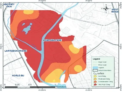
being stationary, omnidirectional (that is isotropic), and show-ing moderate spatial dependency, simple krigshow-ing was used to in-terpolate the surface and was subsequently classified according to the Cdeg categories. Figure 2 shows the spatial distribution

and extent at which AEPS is contaminated. For the purpose of examining the Cdeg, the kriged surface was reclassified according

to the Cdeg set by Meza-Figueroa et al. [16]. The red areas in

Fig-ure 2 indicate highly contaminated sites within the study area. Based on the cluster of areas such as burning, dismantling, rec-reational, residential, etc., an assessment of the Cdeg within AEPS

is presented in Table 4. Table 4 shows mean heavy metal con-centrations in ppm and the Cdeg per site. With reference to the

Cdeg caused by heavy metals per site, the result indicates

burn-Figure 2. Spatial distribution map for degree of contamination (Cdeg).

Table 4. Degree of contamination (Cdeg) and mean concentration of heavy metals per site in AEPS

Site Ba Cd Co Cr Cu Hg Ni Pb Zn Cdeg Burning 641.5 10.1 43.8 171.5 2967.8 3.5 21.8 2666.4 1887.2 393.4 Dismantling 785.7 7.8 66.1 419.2 1643.5 1.6 44.6 846.8 1939.2 193.5 Residential 658.1 2.6 51.5 153.9 1354.6 1.6 27.2 896.1 1170.4 152.2 Recreational 443.7 1.9 36.5 338.6 762.9 0.5 14.8 355.2 700.3 74.2 Commercial area 493.6 0.6 29.6 290.9 157.7 0.3 6.2 163.9 516.9 36.2 Worship 783.9 0.3 30.5 184.6 118.2 0.4 4.9 117.0 419.9 29.4 Farm 315.4 0.2 23.7 319.2 91.4 0.5 4.9 143.5 271.2 29.1 School 394.3 0.3 42.3 118.8 47.6 0.6 2.2 111.3 293.2 25.9 Clinic 581.1 - 28.5 119.3 40.7 - - 55.8 220.5 12.0 Concentration values are measured in ppm.

AEPS, Agbogbloshie electronic waste processing site; Ba, barium; Cd, cadmium; Co, cobalt; Cr, chromium; Cu, copper; Hg, mercury; Ni, nickel; Pb, lead; Zn, zinc.

(6)

ing > dismantling > residential > recreational > commercial area>worship > farm> school> clinic in a descending order of degree or extent of heavy metal contamination. The extremely high values recorded for the burning and dismantling sites could be due to the intensity of activities by informal e-waste recyclers in these areas; a similar trend was reported by previous studies [22–25]. The remaining sequence/order is residential> recre-ational> commercial> worship > farm> school> clinic could be attributed to the proximity of these areas to the main burning and dismantling sites of informal recyclers.

Discussion

The CF shows the contribution of each of the heavy metals to the Cdeg; it shows Zn, Cu, Hg, Cd, and Pb in an increasing order

as contributing immensely to the Cdeg. The kriged map for the

Cdeg estimated on the basis of the CF and reference or

back-ground values is consistent with similar studies [7,16,18,26]. The Cdeg map showed most of the areas within AEPS, which

consists of burning, dismantling, residential, recreational, com-mercial, worship centers, and school were highly or severely contaminated with the studied heavy metals. A further assess-ment of the spatial distribution map revealed 66%, representing 110 ha of the land area, classified as severely contaminated, while 25% (42 ha), 8% (14 ha), and less than 1% classified as considerably, moderately, and slightly contaminated, respective-ly. The significantly high Cdeg, spatial autocorrelation, and spatial

random variance in the Cdeg indicate anthropogenic influence,

i.e., e-waste recycling activities. Hereby, school, residential, mar-ket, farm, and worship areas are of particular concern as children spend a considerable amount of time there. Heavy metals, in particular Pb and Cd, can cross the blood brain barriers of chil-dren, exerting toxic or hazardous effects which might result in a low IQ and developmental disorders; in children and adults, heavy metals can also cause cancer [7,27,28].

The spatial assessment of soil contamination from an informal e-waste recycling site in Agbogbloshie was undertaken by exam-ining levels of heavy metals and the spatial extent of heavy metal contamination as possible environmental impacts of e-waste re-cycling activities. The study concludes that nine heavy metals, namely Ba, Cd, Co, Cr, Cu, Hg, Ni, Pb, and Zn were ubiquitous within AEPS and that heavy metal concentrations in soils from the study exceeded the optimal and action requiring limits of both the Dutch and Canadian SQGV by 10 to 1000 times. These high heavy metal concentrations indicate pollution of AEPS with these nine heavy metals, in particular with Cd, Cu, Hg, Pb, and Zn. In addition, kriging requirements of normality, spatial variation, and autocorrelation were met before

predic-tion of spatial distribupredic-tion maps, which revealed the contamina-tion of the study area to an extent beyond just the main working areas of dismantling and burning sites to areas close to schools, the clinic, residential, and worship premises. The concentra-tions of these heavy metals and the spatial extent of their distri-bution poses an ecological risk for humans and other terrestrial and aquatic species at AEPS; therefore, further research of po-tential ecological and human health risks of informal e-recycling is needed.

Acknowledgements

We sincerely thank the Centre for Development Research, University of Bonn, for funding the data collection and labora-tory analysis of the soil samples. We also thank the Ghana Atomic Energy Commission and the Geological Surveys De-partment, Accra, Ghana, for conducting the laboratory analyses. The Katholischer Akademischer Ausländer-Dienst and the Catholic University College of Ghana provided a monthly sti-pend to Vincent Nartey Kyere.

Conflict of Interest

The authors have no conflicts of interest associated with the material presented in this paper.

ORCID

Vincent Nartey Kyere http://orcid.org/0000-0002-8727-6442

References

1. Yang Y, Williams E. Logistic model-based forecast of sales and gen-eration of obsolete computers in the U.S. Technol Forecast Soc Change 2009;76(8):1105–1114.

2. Yu J, Williams E, Ju M, Yang Y. Forecasting global generation of ob-solete personal computers. Environ Sci Technol 2010;44(9):3232-3237.

3. Solving the E-waste Problem. Annual report 2013/ 2014 [cited 2015 Jun 22]. Available from: http://www.step-initiative.org/files/ step-2014/Publications/Step_ARs/2013_14/step(1)/flipview-erxpress.html.

4. United Nations Environment Programme. E-waste, the hidden side of IT equipment’s manufacturing and use; 2005 [cited 2015 Jun 22]. Available from: http://www.grid.unep.ch/products/3_Re-ports/ew_ewaste.en.pdf.

5. Lundgren K. The global impact of e-waste: addressing the chal-lenge. Geneva: International Labour Office; 2012, p. 72.

6. Caravanos J, Clark E, Fuller R, Lambertson C. Assessing worker and environmental chemical exposure risks at an e-waste recycling and disposal site in Accra, Ghana. J Health Pollut 2011;1(1):16-25.

(7)

7. Atiemo SM, Ofosu FG, Aboh IK, Kuranchie-Mensah H. Assessing the heavy metals contamination of surface dust from waste electri-cal and electronic equipment (e-waste) recycling site in Accra, Ghana. Res J Environ Earth Sci 2012;4(5):605-611.

8. Otsuka M, Itai T, Asante KA, Muto M, Tanabe S. Trace element contamination around the e-waste recycling site at Agbogbloshie, Accra City, Ghana. Interdiscip Stud Environ Chem Environ Pollut Ecotoxicol 2012;6:161-167.

9. Asante KA, Agusa T, Biney CA, Agyekum WA, Bello M, Otsuka M, et al. Multi-trace element levels and arsenic speciation in urine of e-waste recycling workers from Agbogbloshie, Accra in Ghana. Sci Total Environ 2012;424:63-73.

10. Itai T, Otsuka M, Asante KA, Muto M, Opoku-Ankomah Y, Ansa-Asare OD, et al. Variation and distribution of metals and metalloids in soil/ash mixtures from Agbogbloshie e-waste recycling site in Accra, Ghana. Sci Total Environ 2014;470-471:707-716.

11. Ministry of Housing, Spatial Planning and Environment. Dutch target and intervention values, 2000 (the new Dutch list) [cited 2016 Jul 11]. Available from: http://www.esdat.net/Environmen- tal%20Standards/Dutch/annexS_I2000Dutch%20Environmen-tal%20Standards.pdf.

12. Cahn MD, Hummel JW, Brouer BH. Spatial analysis of soil fertility for site-specific crop management. Soil Sci Soc Am J 1994; 58(4):1240-1248.

13. Kerry R, Oliver MA. Average variograms to guide soil sampling. Int J Appl Earth Obs Geoinf 2004;5(4):307–325.

14. Caeiro S, Costa MH, Ramos TB, Fernandes F, Silveira N, Coimbra A, et al. Assessing heavy metal contamination in Sado Estuary sedi-ment: an index analysis approach. Ecol Indic 2005;5(2):151–169. 15. Ott WR. Environmental indices: theory and practice. Ann Arbor:

Ann Arbor Science; 1978.

16. Meza-Figueroa D, De la O-Villanueva M, De la Parra ML. Heavy metal distribution in dust from elementary schools in Hermosillo, Sonora, México. Atmos Environ 2007;41(2):276–288.

17. Muller G. Index of geoaccumulation in sediments of the Rhine River. Geol J 1969;2(3):108–118.

18. Taylor SR, McLennan SM. The continental crust: its composition and evolution. Geol Mag 1985;122(6):673–674.

19. Hakanson L. An ecological risk index for aquatic pollution control. A sedimentological approach. Water Res 1980;14(8):975-1001. 20. Loska K, Cebula J, Pelczar J, Wiechuła D, Kwapuliński J. Use of

en-richment and contamination factors together with geoaccumulation indexes to evaluate the content of Cd, Cu, and Ni in the Rybnik wa-ter reservoir in Poland. Wawa-ter Air Soil Pollut 1997;93(1): 347–365. 21. Loska K, Wiechuła D, Korus I. Metal contamination of farming

soils affected by industry. Environ Int 2004;30(2):159-165. 22. Liu WH, Zhao JZ, Ouyang ZY, Söderlund L, Liu GH. Impacts of

sewage irrigation on heavy metal distribution and contamination in Beijing, China. Environ Int 2005;31(6):805-812.

23. Leung A, Cai ZW, Wong MH. Environmental contamination from electronic waste recycling at Guiyu, southeast China. J Mater Cy-cles Waste Manag 2006;8(1):21–33.

24. Wong CS, Wu SC, Duzgoren-Aydin NS, Aydin A, Wong MH. Trace metal contamination of sediments in an e-waste processing village in China. Environ Pollut 2007;145(2):434-442.

25. Wong CS, Duzgoren-Aydin NS, Aydin A, Wong MH. Evidence of excessive releases of metals from primitive e-waste processing in Guiyu, China. Environ Pollut 2007;148(1):62-72.

26. Leung AO, Duzgoren-Aydin NS, Cheung KC, Wong MH. Heavy metals concentrations of surface dust from e-waste recycling and its human health implications in southeast China. Environ Sci Technol 2008;42(7):2674-2680.

27. Lu X, Wang L, Lei K, Huang J, Zhai Y. Contamination assessment of copper, lead, zinc, manganese and nickel in street dust of Baoji, NW China. J Hazard Mater 2009;161(2-3):1058-1062.

28. Frazzoli C, Orisakwe OE, Dragone R, Mantovani A. Diagnostic health risk assessment of electronic waste on the general popula-tion in developing countries’ scenarios. Environ Impact Assess Rev 2010;30(6):388–399.

29. Riederer AM, Adrian S, Kuehr R. Assessing the health effects of in-formal e-waste processing. J Health Pollut 2013;3(4):1-3.

(8)

(9)

Figure S2. Steps involved in statistical and geostatistical data analysis.

Preparation & data loading

Indicator kriging

Cross validation

Ordinary kriging

Exploratory data analysis

Trend analysis of data

Variogram & semivariogram construction

(10)