A Control Chart for Gamma Distribution using
Multiple Dependent State Sampling
Muhammad Aslam*
Department of Statistics, Faculty of Sciences, King Abdulaziz University, Jeddah, Saudi Arabia Osama-H. Arif
Department of Statistics, Faculty of Sciences, King Abdulaziz University, Jeddah, Saudi Arabia Chi-Hyuck Jun
Department of Industrial and Management Engineering, POSTECH
(Received: May 18, 2016 / Revised: August 31, 2016 / Accepted: September 27, 2016) ABSTRACT
In this article, a control chart based on multiple dependent (or deferred) state sampling for the gamma distributed qual-ity characteristic is proposed using the gamma to normal transformation. The proposed control chart has two pairs of control limits, which can be determined by considering the in-control average run length (ARL). The shift in the scale parameter of a gamma distribution is considered and the out-of-control ARL is evaluated. The performance of the proposed chart has been shown for different levels of the parameters of the proposed control chart. It is also shown that the proposed chart is better than the Shewhart chart in terms of ARLs. A case study with a real data has been in-cluded for the practical usage of the proposed scheme.
Keywords: Multiple Dependent states, Control Chart, Gamma Distribution, Wilson-Hilferty Transformation, Average Run Length, Simulation
* Corresponding Author, E-mail: [email protected]
1. INTRODUCTION
A control chart is an important tool of statistical process control for monitoring and improving the quality of products of any manufacturing process. The idea of control chart was rooted by Shewhart A. Walter during 1920s in Bell Telephone Laboratories. Several modifica-tions have been introduced since its existence but the ba-sic idea of plotting the statistic on the graph of lower and upper limits remains unchanged. It becomes necessary for quality engineers to evaluate the control chart in use whether it has the ability of early detection of the out-of-control process. Early and quick detection of the assigna-ble causes of the on-line process is the prime purpose behind constructing the control charts.
The concept of multiple dependent (or deferred) state
(MDS) sampling was initiated by (Wortham and Baker, 1976). Balamurali and Jun (2007) presented a variable acceptance sampling plan using the MDS scheme and concluded that this sampling scheme is better in risk pro-tection to the manufacturer and the consumer as com-pared to the conventional single and double sampling plans. (Aslam et al., 2015) studied the MDS schemes in the area of acceptance sampling plans and argued that the MDS sampling performs better than the conventional single sampling plans in terms of average sample number. Under the MDS scheme the decision about the in-control or the out-of-control process is made considering the re-sults of the previous samples. If we select a sample from the on line process and posted it on the control chart, then it may fall in any of three mutually exclusive states i.e., in-control state, out-of-control state or the state in which Vol 16, No 1, March 2017, pp.109-117 https://doi.org/10.7232/iems.2017.16.1.109
the decision depends on the previous samples. The MDS sampling have been studied by many authors including among others (Soundararajan and Vijayaraghavan, 1990).
Most of the control charts have been studied assum-ing that the specific quality characteristics of the manu-facturing process follow the normal distribution. But there are situations when the specific quality characteristic does not follow the normal distribution. According to Santiago and Smith (2013) the data not collected in subgroups or a skewed data may not produce good results under the normal distribution. Schilling and Nelson (1976) and Stoumbos and Reynolds Jr (2000) have suggested alterna-tive methods when the quality characteristic of interest follows a skewed distribution. Santiago and Smith (2013) proposed control chart for exponential distribution and named it as t-chart. Santiago and Smith (2013) used trans-formation given by Johnson and Kotz (1970) and Nelson (1994). Mohammed (2004) and Mohammed and Laney (2006) applied t-chart in healthcare. Aslam et al. (2016) proposed t-chart using process capability index. For a skewed distributed quality characteristic, a popularly used distribution to study the phenomena is a gamma distribu-tion. The gamma distribution is frequently used in model-ing the waitmodel-ing time of the life events (Hogg and Craig, 1970; Aksoy, 2000). Al-Oraini and Rahim (2002) worked for economical X-bar chart for gamma distribution. Jearkpaporn et al. (2003) designed control chart for gamma distribution using generalized linear model. Sheu and Lin (2003) used the gamma distribution to study a small shift in the process. Aslam et al. (2014) used the Wilson-Hilferty transformation to propose a control chart for an exponential distribution. Zhang et al. (2007) proposed control chart for gamma distribution.
By exploring the literature and according to the best of author knowledge, there is no work on the designing the control chart for a gamma distribution using MDS sampling. Therefore, this study proposes a new control chart for a gamma distribution using MDS sampling. The rest of the paper is organized as follows: In Section 2 the design of the proposed control chart has been explained. Section 3 explains the performance evaluation of the pro-posed chart in terms of the average run lengths. In Section 4 the comparison of the proposed chart with the Shewhart chart has been described and a simulation study is per-formed to demonstrate the merit of the proposed control chart. A case study with a real data is also added in this section. In Section 5 some conclusions and findings have been explained.
2. DESIGN OF PROPOSED CONTROL CHART The proposed control chart utilizes a gamma to nor-mal approximation under the Wilson-Hilferty transforma-tion. Let T be a random variable from a gamma
distribu-tion with shape parameter ‘a’ and scale parameter ‘b’. The cumulative distribution function (cdf) of the gamma distribution is given by
(
)
t j b a 1 j 1 t e ( b) P T t 1 j! − − = ≤ = −∑
(1)The Wilson and Hilferty (1931) suggested that the transformed variable of T∗ T / is distributed
ap-proximately as normal with mean
* 1/3 T b Γ(a 1 / 3) Γ(a) μ = + (2) and variance * * 2/3 2 T T b Γ(a+2 / 3) μ Γ(a) σ = − (3)
This suggests that T∗is symmetric in distribution, so
a control chart can be designed with the usual upper con-trol limit (UCL) and lower concon-trol limit (LCL). Therefore, we propose the following steps for the development of the control chart for a gamma distributed quality characteris-tic:
Step 1: Select an item randomly and measure its quality characteristic T. Then, calculate T∗:
* 1/3
T =T
Step 2: Declare the process as in-control if LCL2≤ *
2
T ≤UCL .Declare the process to be out-of-control if *
1
T ≥UCL or *
1
T ≤LCL.Otherwise, go to Step-3. Step-3: Declare the process is in-control if i pro-ceeding subgroups have been declared as in-control. Oth-erwise, declare the process to be out-of-control.
The proposed control chart is based on two pairs of control limits, that is the outer control limits of (LCL1,
1
UCL ) and the inner control limits of ( LCL , UCL ) as well as the parameter i. The outer control limits are given by * * * 1/3 0 1 T 1 T 2/3 2 0 1 T b Γ(a 1 / 3) LCL k Γ(a) b Γ(a+2 / 3) k Γ(a) μ σ μ + = − = − − (4a) * * * 1/3 0 1 T 1 T 2/3 2 0 1 T b Γ(a+1ٛ UCL k Γ(a) b Γ(a+2 / 3) k Γ(a) μ σ μ = + = + − (4b)
* * * 1/3 0 2 T 2 T 2/3 2 0 2 T b Γ(a 1 / 3) LCL k Γ(a) b Γ(a+2 / 3) k Γ(a) μ σ μ + = − = − − (5a) * * * 2 T 2 T 1/3 2/3 2 0 0 2 T UCL k b Γ(a 1 / 3) b Γ(a+2/3) k Γ(a) Γ(a) μ σ μ = + + = + − (5b)
In above, k1and k2 are control coefficient to be determined by considering the in-control ARLs while b is the scale parameter when the process is in control. The proposed plan reduces to the traditional Shewhart control chart when the control coefficients k1=k2=kand i 1= .
The control limits can also be written as follows 1/3 1 0 1 LCL =b LL 1/3 1 0 1 UCL =b UL 1/3 2 0 2 LCL =b LL and 1/3 2 0 2 UCL =b UL where 2 1 1
Γ(a+1 / 3) Γ(a+2 / 3) Γ(a+1 / 3)
LL k
Γ(a) Γ(a) Γ(a)
⎡ ⎛ ⎞ ⎤ ⎢ ⎥ = − − ⎜ ⎟ ⎢ ⎝ ⎠ ⎥ ⎣ ⎦ (6a) 2 1 1
Γ(a 1 / 3) Γ(a 2 / 3) Γ(a 1 / 3)
UL k
Γ(a) Γ(a) Γ(a)
⎡ + + ⎛ + ⎞ ⎤ ⎢ ⎥ = + − ⎜ ⎟ ⎢ ⎝ ⎠ ⎥ ⎣ ⎦ (6b) 2 2 2
Γ(a+1 / 3) Γ(a+2 / 3) Γ(a 1 / 3)
LL k
Γ(a) Γ(a) Γ(a)
⎡ ⎛ + ⎞ ⎤ ⎢ ⎥ = − − ⎜ ⎟ ⎢ ⎝ ⎠ ⎥ ⎣ ⎦ (7a) and 2 2 2
Γ(a+1 / 3) Γ(a+2 / 3) Γ(a+1 / 3)
UL k
Γ(a) Γ(a) Γ(a)
⎡ ⎛ ⎞ ⎤ ⎢ ⎥ = + − ⎜ ⎟ ⎢ ⎝ ⎠ ⎥ ⎣ ⎦ (7b)
The probability of declaring as in-control for the proposed control chart when the process is actually in control is given as follows
(
)
0 * in 2 2 0 P =P LCL ≤T ≤UCL b| (8)(
) (
)
{
* *}
1 2 0 2 1 0 P LCL T LCL | b P UCL T UCL | b + < < + < <(
)
{
}
i * 2 2 0 P LCL <T <UCL | b Here,(
) (
)
(
)
* * 2 2 0 2 0 * 2 0 P LCL T UCL | b P T UCL | b P T LCL | b ≤ ≤ = < − <(
)
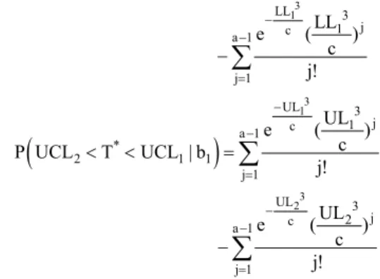
23 3 2 UL 3 j a 1 * 2 2 2 0 j 1 LL 3 j a 1 2 j 1 e (UL ) P LCL T UCL | b j! e (LL ) j! − − = − − = ≤ ≤ = −∑
∑
(
)
23 3 1 LL 3 j a 1 * 2 1 2 0 j 1 LL 3 j a 1 1 j 1 e (UL ) P LCL T LCL | b j! e (LL ) j! − − = − − = < < = −∑
∑
(
)
13 3 2 UL 3 j a 1 * 1 2 1 0 j 1 UL 3 j a 1 2 j 1 e (UL ) P UCL T UCL | b j! e (UL ) j! − − = − − = < < = −∑
∑
The average run length (ARL) for the in-control process is given as follows
0 0 inٛ 1 ARL 1 P = − (9)
Now, we will work for the shifted process. We as-sumed that the scale parameter of the gamma distribution is shifted from b0 to b1when the process is shifted. Let us assume that b1=cb0, where b1 is the shifted scale parame-ter of the gamma distribution and c is the shift constant. Then, the probability of declaring in-control when the process is shifted is given by 1
(
*)
in 2 2 1 P =P LCL ≤T ≤UCL | b(
) (
)
{
* *}
1 2 1 2 1 1 P LCL <T <LCL | b +P UCL <T <UCL | b +(
)
{
}
i * 2 2 1 P LCL ≤T ≤UCL | b Here,(
) (
)
(
)
* * 2 2 1 2 1 * 2 1 P LCL T UCL | b P T UCL | b P T LCL | b ≤ ≤ = < − <(
)
3 2 3 2 UL 3 j 2 c a 1 * 2 2 1 j 1 LL 3 j 2 c a 1 j 1 UL e ( ) c P LCL T UCL | b j! LL e ( ) c j! − − = − − = ≤ ≤ = −∑
∑
(
)
3 2 LL 3 j 2 c a 1 * 1 2 1 j 1 UL e ( ) c P LCL T LCL | b j! − − = < < =∑
3 1 LL 3 j 1 c a 1 j 1 LL e ( ) c j! − − = −
∑
(
)
3 1 3 2 UL 3 j 1 c a 1 * 2 1 1 j 1 UL 3 j 2 c a 1 j 1 UL e ( ) c P UCL T UCL | b j! UL e ( ) c j! − − = − − = < < = −∑
∑
The ARL for the shifted process ARL1 is given as
follows 1 1 in 1 ARL 1 P = −
3. PERFORMANCE EVALUATION OF THE PROPOSED CHART
The performance indicator of any control chart can be best examined and evaluated by the average run length (ARL). Traditionally, the ARL is defined as the average number of samples before the process shows an out-of-control signal (Montgomery, 2007). A greater value of ALR is required when the process is stable and a smaller value is desirable when the process is shifted or out of control. The simulation approach has been used for esti-mating the ARL with the help of the R-language software. This simulation approach is commonly used when the exact form of the mean and other measures of the pro-posed process is not available. Many researchers have used the simulation approach for the effectiveness of con-trol charts including among others Santos (2009), Abbasi and Miller (2013), Ahmad et al. (2013), Ahmad et al. (2013), Chananet et al. (2014), Shu et al. (2014), Aslam et al. (2015), Azam et al. (2015) and Aslam (2016).
The ARL1 values of the shifted process for r0 =
200, 300 and 370, for different shift levels c and five val-ues of the shape parameter a = 1, 2, 5, 10 and 20 are given in Table 1-Table 6. Table 1-Table 3 are for I = 2 and Table 4-Table 6 are for i = 3. As mentioned earlier that the shift occurs in the scale parameter as b1=cb0 when all other
settings are held constants, the decreasing pattern of the ARL1 shows the performance of the proposed chart. From
Table 1~Table 6, we note following trends in control chart parameters.
1. For all other same parameters, as r0 increases
from 200 to 370, the values of ARL increases. 2. For all other same parameters, as a increases
from 2 to 10, the values of ARL1 decreases.
3. For all other same parameters, as i increases from 2 to 3, the values of ARL1 decreases.
Table 1. The ARL1 values for the proposed chart with
i 2= when 200r0= c a 2= a 5= a 10= a 20= 1 k =3.2826 k1=4.4368 k1=5.6645 k1=7.2235 2 k =2.8863 k2=4.0851 k2=5.1897 k2=6.7783 1.00 200.25 200.00 200.00 200.08 1.01 187.12 182.24 175.85 168.34 1.02 175.09 166.40 155.09 142.29 1.03 164.05 152.23 137.19 120.82 1.04 153.90 139.53 121.71 103.04 1.05 144.55 128.13 108.28 88.27 1.10 107.55 85.86 62.83 43.34 1.15 82.16 59.84 38.78 23.46 1.20 64.22 43.17 25.30 13.87 1.30 41.63 24.54 12.42 6.09 1.40 28.80 15.37 7.14 3.41 1.50 20.99 10.42 4.65 2.30 1.60 15.97 7.53 3.34 1.75 1.70 12.59 5.73 2.59 1.47 1.80 10.22 4.56 2.12 1.30 1.90 8.51 3.75 1.82 1.20 2.00 7.23 3.19 1.62 1.13 2.50 4.02 1.88 1.19 1.02 3.00 2.82 1.45 1.07 1.00
Table 2. The ARL1values for the proposed chart with
i 2= when r0=300 c 2 a= a=5 a=10 a=20 1 3.3913 k = k1=4.59934 k1=5.78228 k1=7.2915 2 3.0756 k = k2=3.978001 k2=5.207946 k2=6.872473 1
ARL s ARL s1 ARL s1 ARL s1
1.00 300.08 300.11 300.28 300.90 1.01 279.54 269.73 261.07 252.13 1.02 260.78 242.99 227.74 212.23 1.03 243.62 219.40 199.31 179.44 1.04 227.89 198.54 174.98 152.38 1.05 213.46 180.04 154.11 129.95 1.10 156.73 113.84 85.34 62.30 1.15 118.30 75.39 50.58 32.83 1.20 91.46 52.02 31.85 18.85 1.30 58.13 27.52 14.77 7.80 1.40 39.51 16.36 8.14 4.14 1.50 28.34 10.67 5.13 2.65 1.60 21.24 7.50 3.60 1.95 1.70 16.51 5.61 2.73 1.58 1.80 13.23 4.40 2.21 1.37 1.90 10.88 3.59 1.88 1.25 2.00 9.14 3.03 1.66 1.16 2.50 4.84 1.79 1.20 1.03 3.00 3.27 1.40 1.07 1.00
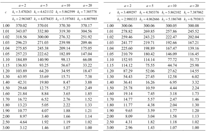
Table 3. The ARL1 values for the proposed chart with i = 2 when r0=370 c 2 a= a=5 a=10 a=20 1 3.470263 k = k1=4.621132 k1=5.862599 k1=7.385778 2 2.963487 k = k2=4.078435 k2=5.197681 k2=6.807985 1.00 370.02 370.01 370.30 370.17 1.01 343.07 332.80 319.30 304.56 1.02 318.56 300.00 276.32 251.92 1.03 296.23 271.03 239.98 209.46 1.04 275.85 245.38 209.14 175.05 1.05 257.23 222.62 182.89 147.04 1.10 184.89 140.90 98.13 66.08 1.15 136.83 93.25 56.67 33.22 1.20 103.89 64.20 34.95 18.47 1.30 63.95 33.69 15.71 7.38 1.40 42.31 19.80 8.47 3.88 1.50 29.68 12.75 5.27 2.49 1.60 21.84 8.84 3.65 1.85 1.70 16.72 6.52 2.76 1.52 1.80 13.23 5.05 2.22 1.33 1.90 10.77 4.07 1.88 1.21 2.00 8.97 3.40 1.66 1.14 2.50 4.64 1.92 1.19 1.02 3.00 3.12 1.46 1.07 1.00
Table 4. The ARL1 values for the proposed chart with i = 3
when r0=200 c 2 a= a=5 a=10 a=20 1 3.282016 k = k1=4.48039 k1=5.655759 k1=7.28655 2 2.944851 k = k2=3.995296 k2=5.262485 k2=6.751103 1.00 200.01 200.03 200.06 200.05 1.01 186.87 180.98 176.05 165.75 1.02 174.83 164.10 155.38 138.08 1.03 163.78 149.10 137.54 115.65 1.04 153.62 135.76 122.09 97.37 1.05 144.27 123.85 108.67 82.41 1.10 107.24 80.51 63.14 38.55 1.15 81.84 54.64 38.97 20.25 1.20 63.91 38.54 25.40 11.80 1.30 41.34 21.19 12.44 5.20 1.40 28.54 13.02 7.16 3.00 1.50 20.77 8.74 4.67 2.09 1.60 15.78 6.31 3.37 1.65 1.70 12.43 4.83 2.62 1.41 1.80 10.08 3.88 2.16 1.27 1.90 8.39 3.23 1.86 1.18 2.00 7.13 2.77 1.66 1.12 2.50 3.99 1.73 1.21 1.02 3.00 2.81 1.38 1.08 1.00
Table 5. The ARL1 values for the proposed chart with i = 3
when r0=300 c 2 a= a=5 a=10 a=20 1 3.409297 k = k1=4.585376 k1=5.862102 k1=7.387062 2 2.988333 k = k2=4.062666 k2=5.186748 k2=6.793813 1.00 300.06 300.06 300.05 300.08 1.01 278.82 269.85 257.86 245.52 1.02 259.46 243.23 222.47 202.04 1.03 241.77 219.71 192.66 167.21 1.04 225.60 198.89 167.47 139.16 1.05 210.79 180.42 146.09 116.45 1.10 152.93 114.14 77.72 51.73 1.15 114.12 75.55 44.74 25.98 1.20 87.29 52.06 27.62 14.55 1.30 54.43 27.45 12.58 6.02 1.40 36.41 16.26 6.95 3.32 1.50 25.78 10.59 4.44 2.24 1.60 19.14 7.45 3.18 1.73 1.70 14.77 5.57 2.47 1.46 1.80 11.77 4.38 2.04 1.30 1.90 9.65 3.59 1.77 1.20 2.00 8.09 3.04 1.58 1.13 2.50 4.31 1.82 1.18 1.02 3.00 2.96 1.43 1.07 1.00
Table 6. The ARL1 values for the proposed chart with i = 3
when r0=370 c 2 a= a=5 a=10 a=20 1 3.480068 k = k1=4.587742 k1=5.79097 k1=7.35734 2 2.982044 k = k2=4.293158 k2=5.372559 k2=6.89495 1.00 370.12 370.18 370.94 370.66 1.01 342.67 334.91 323.42 306.42 1.02 317.74 303.64 282.86 254.53 1.03 295.05 275.88 248.13 212.43 1.04 274.37 251.15 218.30 178.12 1.05 255.50 229.10 192.60 150.04 1.10 182.42 148.71 107.22 68.01 1.15 134.14 100.61 63.52 34.26 1.20 101.24 70.58 39.81 19.02 1.30 61.66 38.10 18.13 7.57 1.40 40.45 22.79 9.77 3.98 1.50 28.18 14.81 6.03 2.57 1.60 20.64 10.31 4.15 1.92 1.70 15.74 7.60 3.11 1.57 1.80 12.43 5.87 2.48 1.37 1.90 10.11 4.72 2.08 1.25 2.00 8.42 3.92 1.82 1.17 2.50 4.39 2.15 1.26 1.03
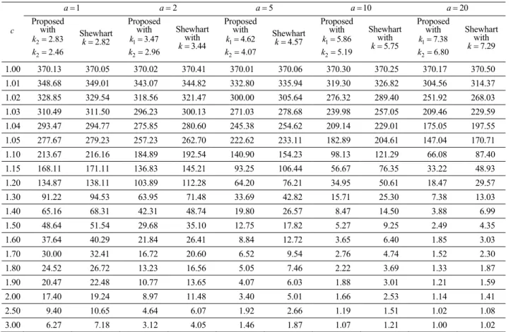
4. ADVANTGES OF PROPOSED CHART As mentioned earlier the proposed control chart is equal to the Shewhart chart when the two control con-stants are equal (k1 = k2) and i = 1. Tables 7 and 8 have
been generated for the ARL1 comparison of the proposed
control chart with the Shewhart chart. The efficiency of the proposed chart can be observed by the decreasing pattern of the ARL1 values; for instance, the ARL1 of the
proposed chart is 147.04 for a = 20 and c = 1.05 whereas the same shift is detected after 170.71 samples on the average for the existing chart as mentioned in Table 7. The efficiency of the proposed chart is checked for all the possible combinations of the different sittings of r0 = 200,
300 and 370, a = 1, 2, 5, 10 and 20 and shift levels c = 1, 1.01, 1.02, 1.03, 1.04, 1.05, 1.1, 1.15, 1.2, 1.3, 1.4, 1.5, 1.6, 1.7, 1.8, 1.9, 2.0, 2.5 and 3.
4.1 Simulation Study
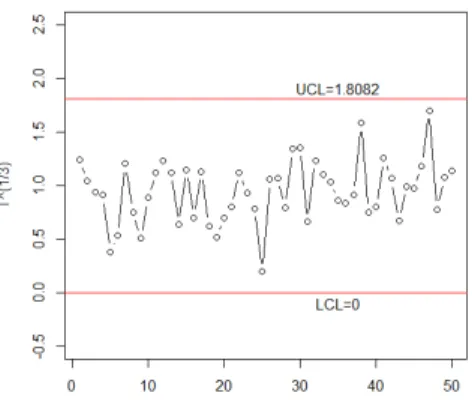
In this section, we will demonstrate the efficiency of the proposed control chart. For this purpose, we will use the simulated data from the gamma distribution. The data is generated and placed in Table 9. The first 20 ob-servations have been generated for in-control process using gamma distribution with a = 2 and b = 1. Next 30
observations have been generated from a shifted parame-ter of b =1.5. Figure 1 shows the proposed control chart with 370 for the simulated data, which indicates the out-of-control process at 49th (or 29th subgroup after
the actual process shift) subgroup.
The Shewhart chart for this data is shown in Figure 2. From this figure, it can be read that all values are with-in the control limits which with-indicates that the process is with-in control. So, we can say that the proposed control chart performs better to detect a shifted process than the Shew-hart cShew-hart.
4.2 Industrial Example
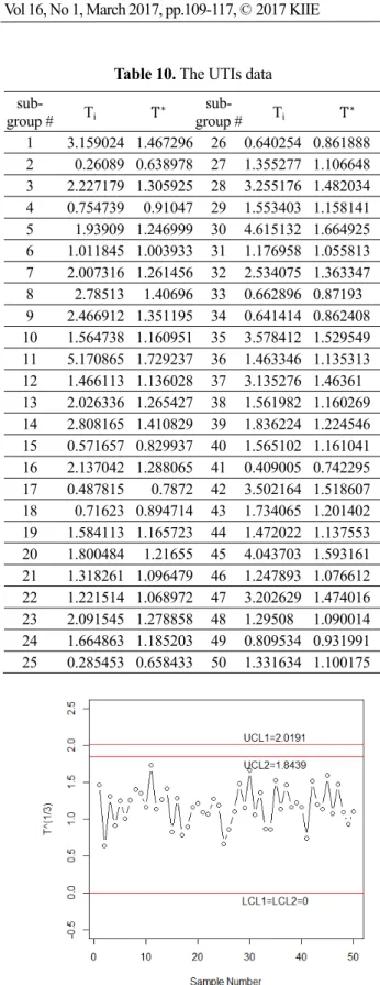
In this section, the proposed control chart is applied to monitoring of urinary tract infections (UTIs) at a large hospital. The data represents the duration of male UTIs patient at a hospital. Similar data was used by Santiago and Smith (2013). The data is known to follow the gamma distribution with shape a = 2. The UTIs data is reported in Table 10.
The control limits of the proposed control chart for UTIs data are given in Figure 3. It can be seen from Figure 3 that the process is in-control although some points are close to UCL2.
Table 7. The Comparison of ARL1 values for proposed chart with i = 2 and Shewhart Chart when r0=370
c 1 a= a= 2 a=5 a=10 a=20 Proposed with 2 2.83 k = 2 2.46 k = Shewhart 2.82 k= Proposed with 1 3.47 k = 2 2.96 k = Shewhart with 3.44 k= Proposed with 1 4.62 k = 2 4.07 k = Shewhart 4.57 k= Proposed with 1 5.86 k = 2 5.19 k = Shewhart with 5.75 k= Proposed with 1 7.38 k = 2 6.80 k = Shewhart with 7.29 k= 1.00 370.13 370.05 370.02 370.41 370.01 370.06 370.30 370.25 370.17 370.50 1.01 348.68 349.01 343.07 344.82 332.80 335.94 319.30 326.82 304.56 314.37 1.02 328.85 329.54 318.56 321.47 300.00 305.64 276.32 289.40 251.92 268.03 1.03 310.49 311.50 296.23 300.13 271.03 278.68 239.98 257.05 209.46 229.59 1.04 293.47 294.77 275.85 280.60 245.38 254.62 209.14 229.01 175.05 197.55 1.05 277.67 279.23 257.23 262.70 222.62 233.11 182.89 204.61 147.04 170.71 1.10 213.67 216.16 184.89 192.54 140.90 154.23 98.13 121.29 66.08 87.40 1.15 168.11 171.11 136.83 145.21 93.25 106.44 56.67 76.35 33.22 48.93 1.20 134.87 138.11 103.89 112.28 64.20 76.21 34.95 50.61 18.47 29.57 1.30 91.22 94.53 63.95 71.48 33.69 42.82 15.71 25.30 7.38 13.03 1.40 65.16 68.31 42.31 48.74 19.80 26.57 8.47 14.50 3.88 6.99 1.50 48.64 51.54 29.68 35.10 12.75 17.82 5.27 9.25 2.49 4.35 1.60 37.64 40.29 21.84 26.41 8.84 12.72 3.65 6.40 1.85 3.03 1.70 30.00 32.41 16.72 20.60 6.52 9.54 2.76 4.74 1.52 2.30 1.80 24.52 26.72 13.23 16.56 5.05 7.46 2.22 3.69 1.33 1.87 1.90 20.47 22.48 10.77 13.65 4.07 6.03 1.88 3.01 1.21 1.59 2.00 17.40 19.24 8.97 11.48 3.40 5.01 1.66 2.53 1.14 1.41 2.50 9.40 10.65 4.64 6.07 1.92 2.66 1.19 1.51 1.02 1.08 3.00 6.27 7.18 3.12 4.05 1.46 1.87 1.07 1.21 1.00 1.02
Table 8. The Comparison of ARL1 values for proposed chart with i = 3 and Shewhart Chart when r0=370 c 1 a= a=2 a=5 a=10 a=20 Proposed with 1 2.84 k = 2 2.45 k = Shewhart with 2.82 k= Proposed with 1 3.48 k = 2 2.98 k = Shewhart with 3.44 k= Proposed with 1 4.58 k = 2 4.29 k = Shewhart with 4.57 k= Proposed with 1 5.79 k = 2 5.37 k = Shewhart with 5.75 k= Proposed with 1 7.35 k = 2 6.89 k = Shewhart with 7.29 k= 1.00 370.00 370.05 370.12 370.41 370.18 370.06 370.94 370.25 370.66 370.50 1.01 348.35 349.01 342.67 344.82 334.91 335.94 323.42 326.82 306.42 314.37 1.02 328.34 329.54 317.74 321.47 303.64 305.64 282.86 289.40 254.53 268.03 1.03 309.82 311.50 295.05 300.13 275.88 278.68 248.13 257.05 212.43 229.59 1.04 292.65 294.77 274.37 280.60 251.15 254.62 218.30 229.01 178.12 197.55 1.05 276.73 279.23 255.50 262.70 229.10 233.11 192.60 204.61 150.04 170.71 1.10 212.29 216.16 182.42 192.54 148.71 154.23 107.22 121.29 68.01 87.40 1.15 166.51 171.11 134.14 145.21 100.61 106.44 63.52 76.35 34.26 48.93 1.20 133.18 138.11 101.24 112.28 70.58 76.21 39.81 50.61 19.02 29.57 1.30 89.56 94.53 61.66 71.48 38.10 42.82 18.13 25.30 7.57 13.03 1.40 63.63 68.31 40.45 48.74 22.79 26.57 9.77 14.50 3.98 6.99 1.50 47.27 51.54 28.18 35.10 14.81 17.82 6.03 9.25 2.57 4.35 1.60 36.43 40.29 20.64 26.41 10.31 12.72 4.15 6.40 1.92 3.03 1.70 28.93 32.41 15.74 20.60 7.60 9.54 3.11 4.74 1.57 2.30 1.80 23.58 26.72 12.43 16.56 5.87 7.46 2.48 3.69 1.37 1.87 1.90 19.63 22.48 10.11 13.65 4.72 6.03 2.08 3.01 1.25 1.59 2.00 16.66 19.24 8.42 11.48 3.92 5.01 1.82 2.53 1.17 1.41 2.50 8.96 10.65 4.39 6.07 2.15 2.66 1.26 1.51 1.03 1.08 3.00 5.97 7.18 2.99 4.05 1.59 1.87 1.10 1.21 1.00 1.02
Figure 1. Proposed control chart for the simulated data.
Figure 2. Shewhart control chart for the simulated data. Table 9. Simulated data
sub-
group # Ti T∗ group # sub- Ti T∗
1 1.809837 1.218652 26 5.399110 1.754314 2 1.237889 1.073727 27 1.761243 1.207646 3 2.039374 1.268135 28 1.621473 1.174816 4 1.077306 1.025132 29 1.778716 1.211627 5 2.252738 1.310902 30 1.135961 1.043409 6 3.140944 1.464491 31 2.161189 1.292898 7 5.128173 1.724464 32 0.992741 0.997574 8 0.651883 0.867075 33 1.788702 1.213890 9 0.266029 0.643146 34 2.516615 1.360209 10 1.808507 1.218354 35 2.205274 1.301630 11 0.469320 0.777123 36 3.354196 1.496912 12 0.547690 0.818173 37 2.424050 1.343323 13 1.468596 1.136669 38 3.245086 1.480501 14 0.916153 0.971231 39 3.191697 1.472337 15 0.312489 0.678597 40 0.820055 0.936011 16 0.605785 0.846135 41 1.511208 1.147558 17 2.490716 1.355527 42 0.751908 0.909330 18 1.408161 1.120859 43 2.193221 1.299254 19 1.760745 1.207532 44 1.379546 1.113214 20 2.356271 1.330684 45 1.011609 1.003855 21 5.000220 1.710001 46 1.469198 1.136825 22 3.078897 1.454784 47 5.851449 1.801999 23 2.470717 1.351889 48 1.592499 1.167777 24 3.092654 1.456947 49 11.11340 2.231596 25 1.467930 1.136497 50 1.558906 1.159507
5. CONCLUDING REMARKS
The control chart for the efficient monitoring of the production process has been developed for the multiple
dependent state sampling scheme under the gamma dis-tribution. The control chart coefficients have been esti-mated for various target in-control ARLs. Numerical tables have been constructed for the ARL0 and ARL1
val-ues. The proposed chart is found to be comparatively ef-fective for the monitoring of process shifts from the ARL comparison. It has been observed from a simulation study that the proposed scheme is effective for the quick re-sponse of the shifted process. A real example is added to explain the application of the proposed chart to a health-care area. This example shows that the proposed control chart can be also used in health monitoring. The proposed scheme can be extended for other non-normal distribu-tions as a future research.
ACKNOWLEDGMENTS
This work was funded by the Deanship of Scientific Research (DSR), King Abdulaziz University, Jeddah, Saudi Arabia. The authors, therefore, acknowledge with thanks DSR technical and financial support. The work by Chi-Hyuck Jun is a part of the project entitled ‘Develop-ment of TCS System on ECO-Ship Technology’, funded by the Ministry of Oceans and Fisheries, Korea.
REFERENCES
Abbasi, S. A. and Miller, A. (2013), MDEWMA chart: An efficient and robust alternative to monitor process dispersion, Journal of Statistical Computation and Simulation, 83(2), 247-268.
Ahmad, L., Aslam, M., and Jun, C.-H. (2013), Designing of X-bar control charts based on process capability index using repetitive sampling, Transactions of the Institute of Measurement and Control, 014233121350 2070.
Ahmad, S., Riaz, M., Abbasi, S. A., and Lin, Z. (2013), On monitoring process variability under double sampling scheme, International Journal of Production Economics, 142(2), 388-400.
Aksoy, H. (2000), Use of gamma distribution in hydro-logical analysis, Turkish Journal of Engineering and Environmental Sciences, 24(6), 419-428.
Al-Oraini, H. A. and Rahim, M. (2002), Economic statistical design of X control charts for systems with Gamma (λ, 2) in-control times, Computers & industrial engineering, 43(3), 645-654.
Aslam, M. (2016), A Mixed EWMA–CUSUM Control Chart for Weibull‐Distributed Quality Characteristics, Quality and Reliability Engineering International. Aslam, M., Azam, M., and Jun, C.-H. (2015), Multiple
dependent state repetitive group sampling plan for Burr XII distribution, Quality Engineering, 1-7. Table 10. The UTIs data
sub-group # Ti T∗ group # sub- Ti T∗
1 3.159024 1.467296 26 0.640254 0.861888 2 0.26089 0.638978 27 1.355277 1.106648 3 2.227179 1.305925 28 3.255176 1.482034 4 0.754739 0.91047 29 1.553403 1.158141 5 1.93909 1.246999 30 4.615132 1.664925 6 1.011845 1.003933 31 1.176958 1.055813 7 2.007316 1.261456 32 2.534075 1.363347 8 2.78513 1.40696 33 0.662896 0.87193 9 2.466912 1.351195 34 0.641414 0.862408 10 1.564738 1.160951 35 3.578412 1.529549 11 5.170865 1.729237 36 1.463346 1.135313 12 1.466113 1.136028 37 3.135276 1.46361 13 2.026336 1.265427 38 1.561982 1.160269 14 2.808165 1.410829 39 1.836224 1.224546 15 0.571657 0.829937 40 1.565102 1.161041 16 2.137042 1.288065 41 0.409005 0.742295 17 0.487815 0.7872 42 3.502164 1.518607 18 0.71623 0.894714 43 1.734065 1.201402 19 1.584113 1.165723 44 1.472022 1.137553 20 1.800484 1.21655 45 4.043703 1.593161 21 1.318261 1.096479 46 1.247893 1.076612 22 1.221514 1.068972 47 3.202629 1.474016 23 2.091545 1.278858 48 1.29508 1.090014 24 1.664863 1.185203 49 0.809534 0.931991 25 0.285453 0.658433 50 1.331634 1.100175
Aslam, M., Azam, M., Khan, N., and Jun, C.-H. (2015), A control chart for an exponential distribution using multiple dependent state sampling, Quality & Quantity, 49(2), 455-462.
Aslam, M., Mohsin, M., and Jun, C.-H. (2016), A New t-Chart Using Process Capability Index, Communi-cations in Statistics-Simulation and Computation (just-accepted).
Azam, M., Aslam, M., and Jun, C.-H. (2015), Designing of a hybrid exponentially weighted moving average control chart using repetitive sampling, The Inter-national Journal of Advanced Manufacturing Tech-nology, 77(9-12), 1927-1933.
Balamurali, S. and Jun, C.-H. (2007), Multiple dependent state sampling plans for lot acceptance based on measurement data, European Journal of Operational Research, 180(3), 1221-1230.
Chananet, C., Sukparungsee, S., and Areepong, Y. (2014), The ARL of EWMA chart for monitoring ZINB model using Markov chain approach, International Journal of Applied Physics and Mathematics, 4(4), 236.
Hogg, R. V. and Craig, A. T. (1970), introduction to. Math-ematical stati sties EDITION.
Jearkpaporn, D., Montgomery, D. C., Runger, G. C., and Borror, C. M. (2003), Process monitoring for correlated gamma‐distributed data using generalized‐linear‐model‐ based control charts, Quality and Reliability Engineer-ing International, 19(6), 477-491.
Johnson, N. L. and Kotz, S. (1970), Distributions in Statistics: Continuous Univariate Distributions: Vol.2: Houghton Mifflin.
Mohammed, M. (2004), Using statistical process control to improve the quality of health care, Quality and Safety in Health Care, 13(4), 243-245.
Mohammed, M. and Laney, D. (2006), Overdispersion in health care performance data: Laney’s approach, Quality and Safety in Health Care, 15(5), 383-384.
Montgomery, D. C. (2007), Introduction to Statistical Quality Control, John Wiley & Sons.
Nelson, L. S. (1994), A control chart for parts-per-million nonconforming items, Journal of Quality Technology, 26(3), 239-240.
Santiago, E. and Smith, J. (2013), Control charts based on the exponential distribution: Adapting runs rules for the t chart, Quality Engineering, 25(2), 85-96. Santos, D. (2009), Beyond Six Sigma: A Control Chart for
Tracking Defects per Billion Opportunities (dpbo), International Journal of Industrial Engineering: Theory, Applications and Practice, 16(3), 227-233.
Schilling, E. G. and Nelson, P. R. (1976), The effect of non-normality on the control limits of X-bar charts, Journal of Quality Technology, 8(4).
Sheu, S. H. and Lin, T. C. (2003), The generally weighted moving average control chart for detecting small shifts in the process mean, Quality Engineering, 16(2), 209-231.
Shu, L., Huang, W., and Jiang, W. (2014), A novel gradient approach for optimal design and sensitivity analysis of EWMA control charts, Naval Research Logistics (NRL), 61(3), 223-237.
Soundararajan, V. and Vijayaraghavan, R. (1990), Con-struction and selection of multiple dependent (deferred) state sampling plan, Journal of Applied Statistics, 17(3), 397-409.
Stoumbos, Z. G. B. and Reynolds Jr, M. R. (2000), Ro-bustness to non-normality and autocorrelation of individuals control charts, Journal of Statistical Com-putation and Simulation, 66(2), 145-187.
Wortham, A. and Baker, R. (1976), Multiple deferred state sampling inspection, The International Journal Of Production Research, 14(6), 719-731.
Zhang, C., Xie, M., Liu, J., and Goh, T. (2007), A control chart for the Gamma distribution as a model of time between events, International Journal of Production Research, 45(23), 5649-5666.