2276
Copyright ⓒ The Korean Institute of Electrical Engineers
Lumped-Parameter Thermal Analysis and Experimental Validation
of Interior IPMSM for Electric Vehicle
Qixu Chen
†and Zhongyue Zou*
Abstract
– A 50kW-4000rpm interior permanent magnet synchronous machine (IPMSM) applied to the high-performance electric vehicle (EV) is introduced in this paper. The main work of this paper is that a 2-D T-type lumped-parameter thermal network (LPTN) model is presented for IPMSM temperature rise calculation. Thermal conductance matrix equation is generated based on calculated thermal resistance and loss. Thus the temperature of each node is obtained by solving thermal conductance matrix. Then a 3-D liquid-solid coupling model is built to compare with the 2-D T-type LPTN model. Finally, an experimental platform is established to verify the above-mentioned methods, which obtains the measured efficiency map and current wave at rated load case and overload case. Thermocouple PTC100 is used to measure the temperature of the stator winding and iron core, and the FLUKE infrared-thermal-imager is applied to measure the surface temperature of IPMSM and controller. Test results show that the 2-D T-type LPTN model have a high accuracy to predict each part temperature.Keywords:
Interior Permanent Magnet Synchronous Machine (IPMSM), Lumped-Parameter Thermal Network (LPTN), Thermal resistance, Thermal conductance.1. Introduction
Thermal analysis of interior permanent magnet synchro-nous machine (IPMSM) is very important at load and overload, especially in the field of electric vehicle (EV) and hybrid electric vehicle (HEV), which requires higher power density and torque density. Therefore, accurate temperature rise calculation becoming increasingly more and more important. [1]
There are three basic analysis methods: 1) the lumped-parameter thermal model, 2) the finite element method (FEM) and 3) computed fluid dynamics (CFD). Mellor et al [2] studied an induction motor using the lumped parameter thermal model to calculate the average temperatures at different parts of the motor. A lumped-parameter thermal network model for radial flux IPMSM [3-5] and axial flux IPMSM [6-7] is used to calculate the average temperatures for different parts of IPMSM. Fluid flowing characteristics including gap air and coolant [8-9] are studied. Coupled electromagnetic and thermal analysis of IPMSM is carried out in the paper [10-14] and a test platform was established by temperature sensor and infrared thermal imager. P.W. Han, et al [14] used analytical lumped-circuit method and compared with the experiment results for a 29kW high speed induction motor at 12,000rpm. C.B. Park [15] conducted thermal analysis of the 110kW IIPMSM using
the 3-D thermal equivalent network with thermal equivalent circuit of the water cooling jacket. M. Polikarpova, et al [16] proposed hybrid cooling arrange-ment and adopted computational fluid dynamics and finite-element analysis for a 100kW AFPM electrical machine. An infrared camera was used to determine temperatures distribution outside the ISG. FEM simulations can be accurate to compute temperature distributions of motor parts, but convection heat transfer coefficients generally use empirical formula, which lead to the uncertainty of results.
An IPMSM is introduced in the paper. Forced liquid (50%water+50% glycol) cooling in shell jacket is adopted. A T-type lumped-parameter thermal network model of IPMSM for thermal design and analysis is presented. This method divided into two stages combines both analytical and CFD simulations. In the first stage, fluid can be modeled using CFD tools, and in this way, heat transfer coefficients can be accurately computed between solid surface and fluid surface, which are necessary for FEM and LPTN model. In the second stage, heat transfer coefficients obtained by CFD simulations can be used to amend the empirical formula. In this way, a simplified model considering its symmetry and period is introduced in this paper. Finally, a temperature rise test platform under the rated load and overload condition is established to verify the above-mentioned lumped-parameter thermal network result and CFD simulation result. Furthermore, a measured efficiency map is obtained at operation region. The temperature measurements of IPMSM are carried out using thermocouple PTC100 and FLUKE infrared-thermal camera device.
† Corresponding Author: Dept. of Electrical Engineering, Xi’an Jiaotong University, China. ([email protected])
** Dept. of Mechanical Engineering, Xi’an Jiaotong University, China. ([email protected])
2. Lumped Parameter Thermal Network
A lumped-parameter thermal network model applied to IPMSM is presented. Each cylindrical component can be described by lumped-parameter thermal network composed of radial resistance, axial resistance and heat source. The definition of thermal resistances in lumped-parameter thermal network is related to thermal conductivity of material and its dimensional information. In this paper, heat transfer mechanisms of IPMSM, which are generally classified as thermal conduction and thermal convection, are discussed in detail. A. B. Nachouane, et al [17] proposed a traditional lumped-parameter thermal network to estimate the temperature distribution for a 6kW integrated starter generator (ISG).2.1 Model and parameter of IPMSM
The principle of volume equivalence is adopted in this paper, in other words, the heat generation rate of heat source components needs to keep unchanged. Flow chart of nodal temperature rise calculation using LPTN method is given in Fig. 1.
Main parameters of IPMSM is shown as in Table 1.
Table 1. IPMSM dimensions and parameters
Parameter Symbol Value Rated power [kW]/speed [rpm] PN/n 50/4000
Stator outer [mm] Do 208
inner diameter [mm] Di 150
Stator iron length [mm] Lef 160
Number of parallel branches a 2 Number of turns per coil Ns 10
Length of air gap [mm] δ 1.5 PM thickness [mm] hpm 6
Number of stator slots/pole pairs Q /p 36/3 Winding connection type ― Y Coolant flow velocity [L/min] V 8
Start Satisfy temperature rise condition? Save results End Compute loss
Compute coefficients of heat conductance and heat transfer
Compute node temperature rise Compute node thermal resistance Generate thermal conductance matrix Establish thermal equilibrium equation Establish T-type
thermal network model
No
Yes Modify
Fig. 1 Flow chart of nodal temperature rise calculation
Heat source components including stator iron, stator winding, rotor shoe, rotor yoke and PM in Fig. 2, can be equivalent to general cylindrical component model according volume equivalence in Fig. 3.
2.2 Thermal resistance definition
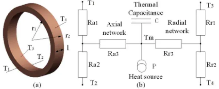
A general cylindrical component and its lumped-parameter thermal network that is derived from the solution of the heat conduction equations are shown in Fig. 4. The
Table 2. Thermal resistance of cylindrical component
R Radial direction Axial direction R1
(
)
2 2 1 2 2 2 1 2 2 ln 1 1 4 r r r r k l r r p é ù -ê ú -ê ú ë û 2 2 1 2 2 a( ) l k r r p -R2 ( ) 2 1 1 2 2 2 1 2 2 ln 1 1 4 r r r r k l r r p é ù -ê ú -ê ú ë û(
)
2 2 1 2 2 a l k r r p -R3 ( )(
)
2 2 1 2 1 2 2 2 1 2 2 2 1 2 2 2 1 2 4 ln 8 r r r r r r r r r r k l r p - - + --(
)
2 2 1 2 6 a l k r r p-Fig. 2. IPMSM geometry model (half model)
Fig. 3. Equivalent model of heat source (half model)
Fig. 4. (a) Cylindrical component (b) Radial and axial
corresponding thermal resistance definition is given in Table 1 [5-7], where kr and ka are the thermal conductivity
in the radial and axial directions respectively; l is the axial length and r2 and r1 are the outer and inner radius
of the cylindrical component; T3 and T4 are the unknown
temperatures on the inner and outer surfaces, and T1 and
T2 are the unknown temperatures at two end face; Tm
represents the average temperature of the component; P and C represent the corresponding internal loss and thermal capacitance. Thermal capacitance in steady state analysis is here under no consideration.
Table 3 gives some typical values for the thermal conductivities of solid materials applied to IPMSM [6].
2.3 Heat conduction and thermal convection
Heat conduction and thermal convection of the fluid including liquid coolant and air are considered in calculating IPMSM temperature rise.
General formula of heat conduction Gmat is shown as
mat mat mat A G L l = (1)
where Gmat is heat conduction, λ is thermal conductivity,
Amat is cross-sectional area, Lmat is path length along the
heat conduction direction.
The equivalent thermal conductance Gmat1,2 with or
without assembly clearance is considered as follows.
1,2 1 2 1,2 1 2 1 1 1 1 1 1 1 mat
mat air mat
mat mat mat G G G G G G G ì = ï + + ï í ï = ï + î (2)
where Gmat1 and Gmat2 are thermal conductance of different
material, Gair is thermal conductance of air.
Most of heat generated by IPMSM parts could be taken away by circulating liquid coolant in shell jacket. Shell jacket includes S-type channel filling with liquid coolant. Pressure loss and wall heat transfer coefficient distribution of shell jacket is obtained by FLUENT in Fig. 5(a), and its equivalent water circuit is shown in Fig. 5(b).
The total loss is the sum of the losses of all parts as shown in
(a)
(b)
Fig. 5. Water channel (a) Pressure loss and wall transfer
coefficient (b) Equivalent water circuit model
losses Cu Fe pm ro air be ex P P P P P P P P Q C T = + + + + + + = × × D (3) 2 2 v Q A = (4)
where Plosses is total loss of IPMSM, PCu is copper loss, PFe
is stator iron loss, Ppm is eddy current loss of PM, Pro is
eddy current loss of rotor, Pair is friction loss of air, Pbe is
bearing loss, Pex is extra loss, V2 is the velocity of the
liquid coolant, Q is the flow of liquid coolant, A2 is the
cross-sectional area of water channel.
As can be seen from Fig. 5, the total pressure loss p of liquid coolant through shell jacket can be expressed by
6 1 2 +n i i p p p = = D ×
å
D (5)(
)
(
)
(
)
(
)
2 2 2 2 3 3 3 3 3 2 2 1 2 2 2 1 1 1 1 2 2 2 2 3.5 2 2 3 3 2 3 2 2 3 2 2 3 2 4 4 5 5 3 2 2 3.5 2 2 6 6 3 2 1 1 1 1 1 ; 2 2 2 2 1 0.131 0.163 2 1 1 1 1 1 ; 1 2 4 2 2 1 0.131 0.163 2 A L p v v p v v A D p v D D v A A p v v p v v A A p v D D v m z r r z r r z r r z r r z r r z r r ì æ ö ïD = = ç - ÷ D = = ï è ø ï D = = + × ï ï í æ ö æ ö D = = ç - ÷ D = = ç - ÷ è ø è ø D = = + × î ï ï ï ï ï (6) where Δp1, Δp4, and Δp5 are pressure loss corresponding tothe changing cross section, Δp2 is the pressure loss along
the water channel, Δp3 and Δp6 are pressure loss due to its
connection with the elbow, n is number of water channel. Thermal conductance between inner wall of shell jacket and liquid coolant is shown by
Table 3. IPMSM thermal parameters
Thermal conductivity Symbol Value Silicon steel [W/(K.m)](x,y,z) λSi (4.5,45,45)
Copper[W/(K.m)] λCu 386
Aluminum alloy [W/(K.m)] λAl 201
Winding insulation [W/(K.m)] λInsu 0.26
PM [W/(K.m)] λpm 8
0.14 1/3 1/3 1/3 2 0.8 0.4 1.86 Re Pr Re<2200 0.023 Re Pr Re>2200 e wa wa wa wa d v Nu L u ì æ ö æ ö ï ç ÷ ç ÷ = í è ø è ø ï î (7) 2 2 2 Re ( ) e wa wa wa d ab v v a b u u = = + (8) Nu wa wa e h D l = (9) wa wa wa G =h ×A (10)
where λwa is the thermal conductivity of liquid coolant,
Nuwa is the Nusselt number of liquid coolant, Rewa is the
Rayleigh number of liquid coolant., Pr is the Prandtl number, de is the equivalent diameter, a is the width of
water channel, b is height of water channel, υwa is kinematic
viscosity coefficient of liquid coolant, hwa is convective
heat transfer coefficient of liquid coolant, L is the path length of water channel.
Thermal conductance Gair1 between rotor end surface
and gap air is shown by (11)-(15). The heat transfer coefficient hair1 of air can be obtained by classical Nusselt number. 1 air Nu h l d × = (11)
The Nusselt number Nu of air is calculated for three different Taylor number Ta as shown in
0.367 4
0.241 4 7
2 for Ta<1700 0.128Ta for 1700<Ta<1 0.409 for 1e <Ta<1e Nu e Ta ì ï = í ï î (12)
where Taylor number Ta and Reynolds number Re are shown as 2 Re Ta r d × = (13) Re v d u × = (14)
where υ is kinematic viscosity of the air (m2/s) and v is linear speed of the rotor (m/s); Thermal conductance Gair1
at air gap is obtained by
1 1 1 o
air air air air
G =h A =h pD L (15)
Heat transfer coefficient hair2 and thermal conductance
Gair2 between the rotating shaft and internal air can be
written as
2 15.5 (0.39 1)
air
h = × v+ (16)
2 2 2
air air air
G =h ×A (17)
Heat transfer coefficient hair3 and thermal conductance
Gair3 at the location of end winding surface can be written
as illustrated by
3 14.2 (1 )
air
h = × +k v (18)
3 3 3
air air air
G =h ×A (19)
where k is the coefficient of the air blowing rate, Aair3 is
surface area of end winding (unit:m2).
The thermal conductance Gair4 and external surface heat
transfer coefficient hair4 between shell and ambient air can
be evaluated as
(
)
1/3 4 14 1 0.5 25 shell air T h = + v æç ö÷ è ø (20) 4 4 4air air air
G =h ×A (21)
where v is wind speed (that is linear speed of shell surface. unit: m/s); Tshell is external surface temperature of shell
(unit: K).Aair4 is surface area of shell (unit:m2).
2.4 Thermal conductance and T–type thermal network
For steady-state thermal analysis, the temperature rise T of each node of lumped-parameter thermal network is calculated as shown in equation (22)-(24), where the dimension of thermal conductance matrix Gnxn is n=34.
G T× =W (22)
( )
(
)
( )
(
)
(
)
(
)
(
)
(
)
( )
(
)
( )
(
)
(
)
(
)
(
)
(
)
1 1 2 2 1,1 1, 2 1,i 1, 2,1 2, 2 2, 2, ,1 , 2 , , ,1 , 2 , , i i n n G G G G n T W T W G G G i G n T W G i G i G i i G i n T W G n G n G n i G n n é - ××× - - ù é ù é ù ê ú ê ú ê ú - ××× - -ê ú ê ú ê ú ê ú ê ú ê ú × = ê- - ××× ××× - ú ê ú ê ú ê ú ê ú ê ú ê ××× ú ê ú ê ú ê- - ××× - ××× ú ë û ë û ë ûM
M
M
M
M
M
O
M
M
M
M
M
M
M
M
O
M
(23)( )
( )
(
)
(
)
(
)
(
)
1, , ( , ) ,1 , 2 , 1 , 1 , n j j i G i i G i j G i G i G i i G i i G i n = ¹ = = + + ××× + - + + + ××× +å
(24)Gauss elimination method, Gauss-Seidel iterative method, Jacobi-Cholesky elimination method, or Conjugate gradient method can be adopted to solve thermal conductance matrix.
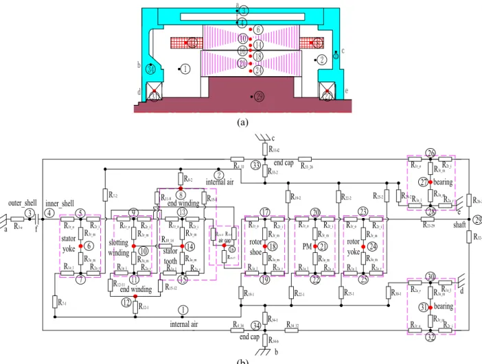
Because of the axial symmetry, only half temperature node distribution drawing of the IPMSM is built in Fig. 6 (a), and the corresponding equivalent T–type LPTN model in Fig. 6(b) in this paper is used for node temperature calculation. The power losses defined in Table IV are injected into the specified thermal nodes of the parts. In the thermal model, the geometry of the IPMSM is divided into the following 18 parts:
1), 2) internal air, 3) outer shell, 4) inner shell, 6) stator yoke, 8), 12) end-winding, 10) slotting winding, 14) stator
teeth, 15) gap air, 18) rotor shoe, 21) magnet, 24) rotor yoke, 27), 31) bearing, 29) shaft, 33), 34) end cap.
Main heat generated by losses is taken away by circulated coolant in shell, therefore, shell is divided into outer shell (3# node) and inner shell (4# node) considering heat convection. Due to the flux density difference between stator tooth (14# node) and stator yoke (6# node), losses of stator tooth and stator yoke are considered separately. Similarly, rotor iron loss fall into rotor shoe (18# node) loss and rotor yoke (24# node) loss.
In order to accurately calculate copper loss, winding is divided into slotting winding (10# node), and two end windings (8# node, 12# node). Bearing (27# node, 31# node) is also considered as a cylindrical component. Non-heat source parts, for example, end cap (33# node, 34# node), shaft (29# node) and shell (3# node, 4# node) are regarded as single node. Friction losses generated by wind are taken into account such as 1# node and 2# node [7].
Table 4 gives loss values for the heat generation applied to IPMSM.
2.5 3-D CFD Verification
B. Zhang, et al [18] adopted computational fluid
Table 4. Loss value of IPMSM parts
Parameter Symbol Value Stator tooth loss [W] PFet 271
Slot winding copper loss [W] PCu1 952
End winding copper loss [W] PCu2 284
Stator yoke loss [W] PFej 428
PM eddy loss [W] Ppm 38
Rotor iron loss [W] Pro 45
Air friction loss [W] Pair 10
Bearing loss [W] Pbe 4
Extra loss [W] Pex 15
Losses values at 50kW power and speed of 4000rpm
Fig. 7. Liquid-solid coupling model
(a)
(b)
74.1 71.1 68.1 65.1 62.0 59.0 56.0 52.9 49.9 46.9 43.9 40.8 37.8 34.8 31.7 28.7
Fig. 8. Temperature distribution of IPMSM (°C)
thermocouple Stator Stator
winding
Stator iron
Rotor iron Rotor
Magnet
Fig. 9. Rotor and stator of IPMSM
Motor controller Load motor Constant temperature cooling tank Power analyzer PMSM Electric parameter sensor box Load motor controller Current clamp Oscilloscope
Fig. 10. Dynamometer platform
Cooling-water machine DC power supply Upper computer console System monitor interface
Fig. 11. Power supply and upper computer console
3. Prototype Manufacture and Test
In order to verify the LPTN model and liquid-solid coupling model, the prototype of IPMSM is manufactured, whose rotor and stator are shown in Fig. 9. A load test platform is established, which mainly include power supply, load motor controller, load motor, electric parameter sensor box, power analyzer, upper computer, IPMSM, controller, constant-temperature cooling tank and cooling-water machine as shown in Fig. 10-Fig. 11.
Measured phase current wave using three AC current clamps at rated load case is obtained in Fig.12, whose peak value reaches 232A.
Measured IPMSM efficiency map in the constant torque
Fig. 12. Phase current wave at rated load
Fig. 13. Efficiency map
Fig. 14. Infrared thermal image of IPMSM at T=119N.m,
and the constant power operating regions is obtained as shown in Fig. 13.
The temperature measurement of IPMSM is carried out using thermocouple PTC100 and a FLUKE infrared-thermal camera device. Thermocouple temperature sensors PTC100 are located into each phase slot windings for measuring winding and iron core temperature. The outer surface temperature including IPMSM and its controller is
measured by using a FLUKE infrared-thermal camera device in Fig. 14-Fig. 15.
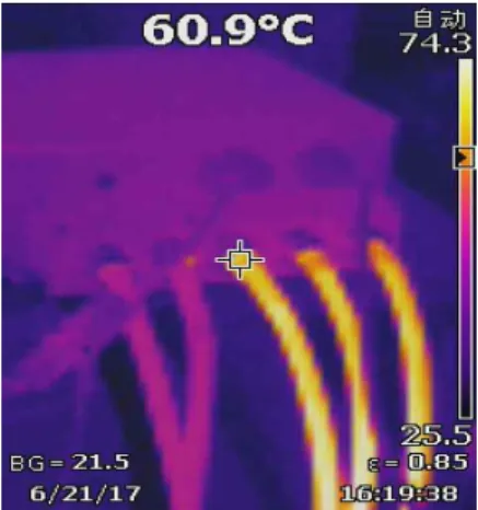
IPMSM phase current at overload case is obtained in Fig. 16, whose peak value reaches 382A. Infrared-thermal image of IPMSM and its controller at overload case are given in Fig. 17-Fig. 18. Power cable temperature of IPMSM and its controller reach 83.9˚C and 60.9˚C respectively.
Comparison among LPTN me thod, CFD method, and experiment results is shown in Table 5, which maintains consistency between experimental results and simulations.
4. Conclusion
Heat transfer coefficients of fluid can be accurately computed using CFD simulation in this paper, which can be used to amend the empirical formula. Therefore, a simplified model considering model symmetry and periodicity is built to reduce the computation time obviously. Assembly clearance between shell and stator iron core is also taken into account. By comparing LPTN result with 3-D liquid-solid coupling CFD result, LPTN method can accurately predict the temperature distribution. Meanwhile, temperature rise test platform including prototype manufacture is built to validate the above two methods using FLUKE infrared-thermal-imager and
Fig. 15. Infrared thermal image of motor controller at
T=119N.m, n=4000rpm, Ia=151A
Fig. 16. Phase current wave at overload case
Fig. 17. Infrared thermal image of IPMSM at T=295N.m,
n=2000rpm, Ia =351A
Fig. 18. Infrared thermal image of motor controller at
T=295N.m, n=2000rpm, Ia =351A
Table 5. Calculated and measured temperature at rated
load
Parameter Method A Method B Method C
Slot winding 74 76 75 Stator iron 60 62 64 Rotor iron 66 68 69 PM 66 67 70 Bearing 42 38 41 Shell 26 29 25 End cap 31 33 30 Shaft extension 34 36 32 A: Lumped-parameter thermal network; B: fluid-solid coupling CFD; C: Measured (50kW, 4000rpm, 151A) [°C]
thermocouple PTC100. The method will be important for practical engineering application.
References
[1] A. Boglietti, A. Cavagnino, D. Staton, M. Shanel, M. Mueller, and C. Mejuto, “Evolution and modern approaches for thermal analysis of electrical machines,”
IEEE Trans. Ind. Electron., vol. 56, no. 3, pp.
871-882, Mar. 2009
[2] P. D. Mellor, D. Roberts, and D. R. Turner, “Lumped parameter thermal model for electrical machines of TEFC design,” Proc. Inst. Electr. Eng, B, vol. 138, no. 5, pp. 205-218, Sep. 1991.
[3] J. Nerg, M. Rilla, and J. Pyrhönen, “Thermal analysis of radial-flux electrical machines with a high power density,” IEEE Trans. Ind. Electron., vol. 55, no. 10, pp. 3543-3554, Oct. 2008.
[4] C. Jungreuthmayer, T. Bauml, O. Winter, M. Ganchev, H. Kapeller, A. Haumer, and C. Kral, “A detailed heat and fluid flow analysis of an internal permanent magnet synchronous machine by means of computa-tional fluid dynamics,” IEEE Trans. Ind. Electron., vol. 59, no. 12, pp. 4568-4578, Dec. 2012.
[5] A. M. EL-Refaie, N. C. Harris, T. M. Jahns, and K. M. Rahman, “Thermal analysis of multibarrier interior PM synchronous machine using lumped parameter model,” IEEE Trans. Energy Convers., vol. 19, no. 2, pp. 303-309, Jun. 2004.
[6] S. T. Scowby, R. T. Dobson, and M. J. Kamper, “Thermal modeling of an axial-flux permanent magnet machine,” Appl. Thermal Eng., vol. 24, pp. 193-207, 2004.
[7] N. Rostami, M.R. Feyzi, J. Pyrhönen, A. Parviainen, and M. Niemela, “Lumped-parameter thermal model for axial flux permanent magnet machines,” IEEE
Trans. Magn., vol. 49, no. 3, pp.1178-1184, Mar. 2013
[8] D. A. Staton and A. Cavagnino, “Convection heat transfer and flow calculations suitable for electric machines thermal models,” IEEE Trans.Ind. Electron., vol. 55, no. 10, pp. 3509-3516, Oct. 2008.
[9] D. A. Howey, P. R. N. Childs, and A. S. Holmes, “Air-gap convection in rotating electrical machines,”
IEEE Trans. Ind. Electron., vol. 59, no. 3, pp.
1367-1375, Mar. 2012.
[10] F. Marignetti,, V. D. Colli, and Y. Coia, “Design of axial flux PM synchronous machines through 3-D coupled electromagnetic thermal and fluid-dynamical finite-element analysis,” IEEE Trans. Ind. Electron., vol. 55, no. 10, pp. 3591-3601, Oct. 2008.
[11] F. Marignetti and V. D.Colli, “Thermal analysis of an axial flux permanent-magnet synchronous machine,”
IEEE Trans. Magn., vol. 45, no. 7, Jul. 2009
[12] G. Zhang, H.Wei, M. Cheng, B. F. Zhang, and X.B. Guo, “Coupled magnetic-thermal fields analysis of
water cooling flux-switching permanent magnet motors by an axially segmented model,” IEEE Trans. Magn., vol. 53, no. 6, 8106504, June 2017.
[13] H. Vansompel, A. Rasekh, A. Hemeida, J. Vieren-deels, and P. Sergeant, “Coupled electromagnetic and thermal analysis of an axial flux PM machine,” IEEE
Trans. Magn., vol. 51, no.11, 8108104, Nov. 2015.
[14] P.W. Han, J. H. Choi, D.J. Kim, Y.D. Chun and D. J. Bang, “Thermal analysis of high speed induction motor by using lumped-circuit parameters,” Journal
of Electrical Engineering & Technology, vol. 10, no.
5, pp. 2040-2045, Sep. 2015.
[15] C.B. Park, “Thermal analysis of IPMSM with water cooling jacket for railway vehicles,” Journal of
Electrical Engineering & Technology, vol. 9, no. 3,
pp. 882-887, May 2014.
[16] M. Polikarpova, P. Ponomarev and P. Lindh, et,al, “Hybrid cooling method of axial-flux permanent-magnet machines for vehicle applications,” IEEE
Trans. Ind. Electron., vol. 62, no. 12, pp. 7382-7390,
Dec. 2015.
[17] A. B. Nachouane, A. Abdelli, G. Friedrich, and S. Vivier, “Numerical study of convective heat transfer in the end regions of a totally enclosed permanent magnet synchronous machine,” IEEE Trans. Ind.
Appl.,vol. 53, no. 4, pp. 3538-3547, Jul/Aug. 2017.
[18] B. Zhang, T. Seidler, R. Dierken, and M. Doppel-bauer, “Development of a yokeless and segmented armature axial flux machine,” IEEE Trans. Ind.
Electron., vol. 63, no. 4, pp. 2062-2071, Apr. 2016.
Qixu Chen He received bachelor’s
degree in mechatronic engineering from North University of China, Taiyuan, China, in 2007, and master’s degree in mechatronic engineering from Xi Dian University, Xi’an, China, in 2010. He is currently working toward a doctor's degree in electric engineering from Xi'an Jiaotong University, Xi’an, Shaanxi, China, His research interests include IPMSM design and drive of the electric vehicle.
Zhongyue Zou He received the B.S.
degree from Shandong University of Technology and the M.S. degree from Shandong University of Science and Technology. He is currently working toward the Ph.D. degree in mechanical engineering from Xi’an Jiaotong University, Xi’an, China. His research interests include energy management and energy manage-ment.
![Table 3 gives some typical values for the thermal conductivities of solid materials applied to IPMSM [6]](https://thumb-ap.123doks.com/thumbv2/123dokinfo/4889637.36706/3.892.462.823.136.454/table-typical-values-thermal-conductivities-materials-applied-ipmsm.webp)