Design of ramp-stress accelerated life test plans for a parallel system with two independent components using masked data

(1)

International Journal of Reliability and Applications Vol. 18, No. 2, pp. 45-63, 2017

Design of ramp-stress accelerated life test plans for a parallel

system with two independent components using masked data

P. W. Srivastava*_{and Savita}

Department of Operational Research, Faculty of Mathematical Sciences, University of Delhi, Delhi 110007, India

Received 01 August 2017; revised 07 December 2017; accepted 27 December 2017

Abstract: In this paper, we have formulated optimum Accelerated Life Test (ALT) plan for a parallel system with two independent components using masked data with ramp-stress loading scheme and Type-I censoring. Consider a system of two independent and non-identical components connected in parallel. Such a system fails whenever all of its components has failed .The exact component that causes the system to fail is often unknown due to cost and time constraint. For each parallel system at test, we observe its system's failure time and a set of component that includes the component actually causing the system to fail. The stress-life relationship is modelled using inverse power law, and cumulative exposure model is assumed to model the effect of changing stress. The optimal plan consists in finding out the optimum stress rate using D-optimality criterion. The method developed has been explained using a numerical example and sensitivity analysis carried out.

Key Words: Accelerated Life Test, D-optimality criterion, Fisher information matrix,

Masked data, Ramp stress

1. INTRODUCTION AND MOTIVATION

Accelerated Life Tests help in inducing early failures in high reliability items that are likely to last for several years; by subjecting them to higher than normal stress conditions, say higher temperature, voltage, pressure etc.. Stress under accelerated condition can be applied using constant-stress, step-stress, progressive-stress, cyclic stress, random-stress, or combinations of such loadings. The choice of a stress loading depends on how the product or unit is used in service and other practical and theoretical limitations (Nelson (1980), Elsayed (1996)). Life tests under accelerated environmental conditions may be fully accelerated or partially accelerated. In fully accelerated life testing all the test units are run at accelerated condition, while in partially accelerated life testing they are run at

*

Corresponding Author.

(2)

46 Design of ramp-stress accelerated life test plans for a parallel system

both normal and accelerated conditions. The term fully accelerated life test has been coined by Bhattacharyya and Soejoeti (1989) and the term partially accelerated life test is due to DeGroot and Goel (1979). The terms accelerated life tests and fully accelerated life tests are used interchangeably in the literature (Nelson (1990)) has discussed the statistical models, test plans and methods of data analyses for the ALT.

Design of accelerated life tests plans under different stress loading schemes has been studied extensively in the literature. See for example, Srivastava and Gupta (2015) and the references therein. However, all these tests are suitable for one unit or component or subsystem of a system.

Srivastava and Savita (2016) have described the optimal accelerated life test plan for a parallel system with two dependent components under ramp-stress loading using time-censored data, and the optimal plan consists in finding out the optimum stress rate using D-optimality criterion. Often, due to certain environmental conditions, the exact cause of system failure might be unknown. Instead, it can be ascertained that the cause of system failure is due to the component which belongs to some subset of the J components of the system. Such type of observation is referred to as being masked, see Usher and Hodgson (1998). Estimation of component reliability in a parallel system using masked life data has been studied by Sarhan and Ei-Bassiouny (2003). The method developed has been explained using a numerical example and sensitivity analysis carried out.

Acronyms

ALT accelerated life test

Avar asymptotic variance

ML maximum likelihood

Cdf cumulative distribution function Pdf probability distribution function GAV generalized asymptotic variance IWD Inverse Weibull distribution Notation

n Total number of test units

i

S Set of component that may cause the system failure

i

T The life time of system i ij

T

The life time of component j in system i j

f (t)

probability distribution function of component j,j=1,2 j

F (t)

cumulative distribution function of component j,j=1,2 ^ Maximum Likelihood estimate

(t)

ε Cumulative Exposure at time t 0

,

1

γ γ

Parameters of the inverse power law,

γ >

₁

0,

− ∞ < γ < ∞

₀

1

(3)

P. W. Srivastava, Savita 47

{ }

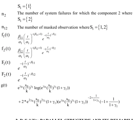
i

S

=

1

2

n

The number of system failures for which the component 2 where

{ }

i

S

=

2

12

n

The number of masked observation where

S

_i

=

{ }

1, 2

1

f (t)

11 11 1 ( 1) ₍ ₎ 11 1 1 t t e β β α β α α − − + ₋ ⎛ ⎞ ⎜ ⎟ ⎝ ⎠ 2

f (t)

12 12 1 ( 1) ₍ ₎ 12 1 1 t t e β β α β α α − − + ₋ ⎛ ⎞ ⎜ ⎟ ⎝ ⎠ 1

F (t)

11 1 ( t ) e β α − − 2

F (t)

12 1 ( t ) e β α − − g(t) ₀ ₁ ₀ ₁ 0 1 0 1 1 0 0 1 1 2 2 0 2 0 1 1 1 1 s s e ( ) log(e ( ) (1 )) k k s s 1 2*e ( ) (1 )(e ( ) (1 )) ( 1 ) k k 1 γ γ γ γ − + γ γ γ γ +γ + γ + + γ + γ − + + γ

2. Reliability PARALLEL STRUCTURE AND ITS RELIABILITY 2.1 Parallel System Configuration

Consider a parallel system that consists of J independent but non-identical components. This system will fail if all of its components failed.

The graphical representation of a parallel system with two components also referred to as a parallel system of order 2 is described in Figure 1.

A

B

Figure 1. Parallel System 2.2 Reliability Function of a Parallel System of order 2

The life time of ith _{parallel system, i = 1, 2, ..., n, with two independent and identical}

components is:

i i1 i2

(4)

where Ti1 and Ti2 represent life times of its components.

The reliability of a parallel system of order 2 is:

0 1 2

F (t) = 1 - F (t)F (t)

. (2) 3. THE MODEL

Assumptions

The following assumptions are made:

a) The system consists of two independent components connected in parallel.

b) It is assumed that the lifetimes of the components have a Weibull distribution with the failure density: 1 ( ; , ) . ⎛ ⎞ − _{−⎜ ⎟} ⎝ ⎠ ⎛ ⎞ = ⎜ ⎟ ⎝ ⎠ x X x g x e β β η β η β η η (3) Here

β

>0 and

η

>0 are the shape and scale parameters. In other words,

( , ) ∼

X WEI

β η

c) There are no any two components failing at the same time. d) Failed parallel systems are not replaced during the test.

e) The occurrence of Masking is independent of the failure cause and time. f) The cumulative exposure model ([5]) holds for the effect of changing stress. g) The inverse power law holds for stress-life relationship, i.e.,

_{( )}

0 1 γ γ s0 s(t) =e s(t) ⎛ ⎞ η _⎜ _⎟ ⎝ ⎠ , (4) where parameters γ0 and γ1 are the characteristics of the product, s(t) is a linear function

of time in ramp-stress, s(t) = kt, where k is the stress rate .

h) The stress applied to test units is continuously increased with constant rate,k, from zero.

3.1 Inverse Weibull (IW) Distribution Under Ramp-Stress The random variableT = 2

X

β _{has the IW distribution. The life distribution and failure} density

of T obtained using (3) are:

( ) ( ; , ) , − − = t T G t e β η

η β

₍₅₎ and ( 1) _{( )} ( ; , ) , − − + ₋ ⎛ ⎞ = _{⎜ ⎟} ⎝ ⎠ t T t g t e β β η β α β η η (6) respectively.

Since the components of a parallel system are assumed to be independent, therefore the joint life distribution of ith system is given by:

(5)

P. W. Srivastava, Savita 49 1 2 1 2 = 1 1 2 2 i i i i T ,T i i T i T i G ( t ,t ) G ( t )G ( t ) 1 1 2 2 1 2 1 2 1 2 − − − − ⇒ = i i i i t t ( ) ( ) T ,T i i G ( t ,t ) e e . β β η η ₍₇₎ The joint pdf of ith_{system is given as:}

1 1 2 2 1 2 1 2 1 2 ( 1) ₍ ₎ ( 1) ₍ ₎ 1 2 1 2 , 1 2 1 1 2 2 ( , ) . − − − + ₋ − + ₋ ⎛ ⎞ ⎛ ⎞ = _⎜ _⎟ _⎜ _⎟ ⎝ ⎠ ⎝ ⎠ i i i i t t i i T T i i t t g t t e e β β β β η η β β η η η η (8)

The stress at time t is from Assumption j is:

s( t ) = kt. (9) From the linear cumulative exposure model and the inverse power law, the joint cdf of the lifetime of ith _{parallel system with independent components under ramp-stress loading is:}

i1 i2 T ,T i1 i2 F (t ,t ) i1 i2 T T i1 i2

= G , (ε(t ),ε(t ))

, (10) whereG( , ) ⋅ ⋅ is the assumed joint inverse cumulative Weibull life distribution function with scale parameter set equal to one, and

0 t

ε(t)= 1 du

η(s(u))

∫ (11) represents the cumulative exposure (damage) model at t.

Since the components are independent, therefore

i1 i2 T ,T i1 i2 F (t ,t ) i1 i2 T i1 T i2

= G (ε(t ))G (ε(t ))

(12) Hence, the cdf and pdf of the lifetime of the ith_{systemunder ramp-stress loading are:}

i1 i2 1 2 i1 i2 0 0 T ,T 1 2 t t du du F ( ) exp[ ( ) ] exp[ ( ) ] 1 1 (s(u)) −β (s(u)) −β = − − η η ∫ _η ∫ _η i1 i2 t ,t 11 12 1 2 1 1 exp[ (( )− ( )− )], = − ti β + ti β α α (13) 11 11 1 2 12 12 ( 1) 1 1 11 , 1 2 1 1 1 ( 1) 2 2 12 1 1 1 ( , ) exp( ( ) ) . exp( ( ) ), − + − − + − ⎛ ⎞ = _⎜ _⎟ − ⎝ ⎠ ⎛ ⎞ − ⎜ ⎟ ⎝ ⎠ i i i i T T i i i i t t f t t t t β β β β β α α α β α α α (14) respectively, where 0 1 1 1 (1 ) 0 1=(e ( ) (1γ s_k γ 1)) +γ

α + γ is the scale parameter,

11 1

(1

1

)

β

=

β

+

γ

and

β

₁₂

=

β

₂

(1

+

γ

₁

)

are the shape parameters. 3.2 Likelihood Function Formulation

(6)

The test procedure consists in putting 'n' independent and identical 2-component parallel systems (parallel systems of order 2) to ramp-stress accelerated test using time-censored (Type-I censored) data. The two components are independent.

The log-likelihood function of n parallel systems of order 2 is obtained as follows: The system will fail if all of its components fail. It means that the system fails at time t_i

if one of its components fails at ti and the rest of the components failed before the time ti

Hence the pdf of lifetime Ti of ith system when a component j, j = 1,2, in the system fails

at time ti and the rest of the components failed before ti is obtained as:

i i ik i i ij i i t 0 _i ik i i ij i i ik i t 0 _i

P[T

t , t

T

t

t ]

lim

t

P[T

t ]P[t

T

t

t | T

t ]

lim

,

t

Δ → Δ →

≤

≤ + Δ

Δ

≤

≤ + Δ

≤

=

Δ

where j ≠ k . Since the components are independent, therefore

i ik i i ij i i t 0 _i

P[T

t , t

T

t

t ]

lim

t

Δ →

≤

≤ + Δ

Δ

_i ik i i ij i i t 0 _i

P[T

t ]P[t

T

t

t ]

lim

t

Δ →

≤

≤ + Δ

=

Δ

=

F (t )f (t )

_{ik i ij i} . Thus, i ik i i ij i i t 0 _i

P[T

t , t

T

t

t ]

lim

t

Δ →

≤

≤ + Δ

Δ

i2 i i1 i i i i1 i i2 i i i

F (t )f (t ) , if component 2 fails before t and component 1 fails at t , and F (t )f (t ) , if component 1 fails before t and component 2 fails at t . ⎧

= ⎨ ⎩

(15)

Using (15), the likelihood function of n parallel systems is:

{ } { } { }

{

}

1 2 12

i i i

n n n

i1 i i2 i i2 i i1 i i1 i i2 i i2 i i1 i

i|S 1 i|S 2 i|S 1,2

L f (t )F (t ) f (t )F (t ) f (t )F (t )+f (t )F (t ) = = = ≡

∏

{ } { } { } 2 _1j 2 _1j i i 11 12 1 2 1 1 j 1 j 1 i i 2 1j i 1j 12 ₁ j 1 i t t ( 1) ( ) ( 1) ( ) n n 11 i 12 i 1 1 1 1 i|S 1 i|S 2 t ( 1) ( ) n 2 1j _i 1 1 j 1 i|S 1,2 t t L e e t e −β −β = = −β = − β + − − β + − α α = = − β + − α = = ⎛ _∑ ⎞ ⎛ _∑ ⎞ ⎜β ⎛ ⎞ ⎟ ⎜β ⎛ ⎞ ⎟ = ⎜_α ⎜_α ⎟ ⎟ ⎜_α ⎜_α ⎟ ⎟ ⎝ ⎠ ⎝ ⎠ ⎜ ⎟ ⎜ ⎟ ⎝ ⎠ ⎝ ⎠ ⎧ _∑ ⎫ β ⎪ ⎛ ⎞ ⎪ × ⎨ _α ⎜_α ⎟ ⎬ ⎝ ⎠ ⎪ ⎪ ⎩ ⎭

∏

∑

∏

(16) ⇒ log-likelihood function is:

(7)

{ }

2 t_i _1j 2 t_i _1j ( ) ( ) ( 1) ( 1) n₁ _t ₁₁ ₁ n₂ _t ₁₂ ₁ j 1 j 1 11 i 12 i

logL log e log e

i|S 1_i 1 1 i|S_i 2 1 1 ⎛ ⎞ ⎛ ⎞ ⎜ ⎟ ⎜ ⎟ ⎛ ⎞ ⎛ ⎞ ⎜ ⎟ ⎜ ⎟ ⎜ ⎟ ⎜ ⎟ ⎜ ⎟ ⎜ ⎟ ⎜ ⎟ ⎜ ⎟ ⎜ _⎝ _⎠ ⎟ ⎜ _⎝ _⎠ ⎟ ⎜ ⎟ ⎜ ⎟ ⎜ ⎟ ⎜ ⎟ ⎝ ⎠ ⎝ ⎠ −β −β − − − β + ∑ _α − β + ∑ _α β ₌ β ₌ = ∑ _{α α} + ∑ _α _α = =

{ }

2 t_i _1j ( ) ( 1) n₁₂ ₂ _t _1j 1 1j i _e j 1 _, j 1 i|S 1,2_i 1 1 ⎧ ⎫ ⎪ ⎪ ⎛ ⎞ ⎪ ⎪ ⎪ _⎜ _⎟ ⎪ ⎨ _⎜ _⎟ ⎬ ⎪ _⎝ _⎠ ⎪ ⎪ ⎪ ⎪ ⎪ ⎩ ⎭ −β − − β + _{∑ α} β ₌ + ∑ _{∑ α α} = = (17)

wheren n= ₁+n₂+n₁₂and n is fixed.

3.3 Parameter Estimation

The MLEs of

γ γ β

₀

,

₁

,

₁and

β

₂are obtained by using NMaximize option of Mathematica 10.0.

3.4 Fisher Information Matrix

It is the 4×4 symmetric matrix of expectation of negative second order partial derivatives of the log likelihood function with respect to γ0, γ1,

β

1and

β

2 .

Thus, the Fisher information matrix F is:

2_L 2_L 2_L 2_L E ₂ E E E 0 1 0 11 0 12 0 2_L 2_L 2_L 2_L E E ₂ E E 1 0 ₁ 1 11 1 22 F F( , ,_{0 1 11 12}, ) 2_L 2 E E 11 0 ⎡ ⎤ _⎡ _⎤ _⎡ _⎤ _⎡ _⎤ ⎢ ⎥ _⎢ _⎥ _⎢ _⎥ _⎢ _⎥ ⎢ ⎥ _⎢ _⎥ _⎢ _⎥ _⎢ _⎥ ⎣ ⎦ ⎣ ⎦ ⎣ ⎦ ⎢ ⎥ ⎣ ⎦ ⎡ ⎤ ⎡ ⎤ ⎡ ⎤ ⎡ ⎤ ⎢ ⎥ ⎢ ⎥ ⎢ ⎥ ⎢ ⎥ ⎢ ⎥ ⎢ ⎥ ⎢ ⎥ ⎢ ⎥ ⎣ ⎦ ⎢_⎣ ⎥_⎦ ⎣ ⎦ ⎣ ⎦ ⎡ ⎤ ⎢ ⎥ ⎢ ⎥ ⎣ ⎦ ∂ ∂ ∂ ∂ − − − − ∂γ ∂γ ∂γ ∂β ∂γ ∂β ∂γ ∂ ∂ ∂ ∂ − − − − ∂γ ∂γ _∂γ ∂γ ∂β ∂γ ∂β ≡ γ γ β β = ∂ ∂ −_{∂β ∂γ} − L E ₂ 2L ₂ E ₂ 2L L / L / 11 1 ₁₁ _{11 22} 2_L 2_L 2_L 2_L E E E E 2 22 0 22 1 22 11 ₂₂ ⎡ ⎤ ⎢ ⎥ ⎢ ⎥ ⎢ ⎥ ⎢ ⎥ ⎢ ⎥ ⎢ ⎥ ⎢ ⎥ ⎢ ⎥ ⎢ ⎥ ⎢ _⎡ _⎤ _⎡ _⎤ ⎥ ⎡ ⎤ ⎢ _⎢ _⎥ _⎢ _⎥ ⎥ ⎢ ⎥ ⎢ _⎢ _⎥ _⎢ _⎥ ⎥ ⎢ ⎥ ⎢ _⎣ _⎦ _⎢ _⎥ _⎢ _⎥ ⎥ ⎣ ⎦ ⎣ ⎦ ⎢ ⎥ ⎢ _⎡ _⎤ ⎥ ⎡ ⎤ ⎡ ⎤ ⎡ ⎤ ⎢ _⎢ _⎥ ⎥ ⎢ ⎥ ⎢ ⎥ ⎢ ⎥ ⎢ ⎥ ⎢ ⎥ ⎢ ⎥ ⎢ ⎥ ⎢ ⎥ ⎢ _⎣ _⎦ _⎣ _⎦ _⎣ _⎦ ⎥ ⎢ ⎥ ⎣ ⎦ ⎣ ⎦ ∂ ∂ − − ∂β ∂γ _∂ _∂β _∂ _{∂β ∂β} ∂ ∂ ∂ ∂ −_{∂β ∂γ} −_{∂β ∂γ} −_{∂β ∂β} − ∂β (18) The calculation of the element of the F in (18) is shown in the Appendix. These elements have been obtained using the following results:

(i)

n

₁ ~ Bin (n, p )₁ , where using (15) 1 i1 i i2 i i 0

p = f (t )F (t )dt

∞

∫

1 1 i 2 i i 0

E[n ] n f (t )F (t )dt

∞

⇒

=

∫

(19)

(8)

52 Design of ramp-stress accelerated life test plans for a parallel system (ii) n₂ ~ Bin (n, p ) ,₂ where using (15) 2 i2 i i1 i i 0

p = f (t )F (t )dt

∞

∫

. 2 2 i 1 i i 0

E[n ] n f (t )F (t )dt

∞

⇒

=

_∫

(20) (iii)

n

₁₂ ~ Bin (n, p )₁₂ , where using (15)

(

)

12 i1 i i2 i i2 i i1 i i 0

p = f (t )F (t ) f (t )F (t ) dt

∞

+

∫

.

(

)

12 1 i 2 i 2 i 1 i i 0

E[n ] n

f (t )F (t ) f (t )F (t ) dt .

∞

⇒

=

∫

+

(21) Since for some set of parameters {

γ γ

₀

, , s , , , k

₁ ₀

β β

_{1 2} }; | F | or variance function may be negative, therefore, we choose only that parametric set for which | F | 0> and variance function, is positive.

4. OPTIMUM PLAN

The optimal plan consists in finding the optimal stress rate using D-optimality criterion wherein the reciprocal of the determinant of F is minimized.a smaller value of the determinant would correspond to a higher (joint) precision of the estimators of parameters (Escobar and Meeker (1995) ).

Thus, the optimization problem is:

Minimize 1 F subject to k> 0.

Optimal k is obtained using the NMinimize option of Mathematica 10.0 .

5. A NUMERICAL ILLUSTRATION AND SENSITIVITY ANALYSIS 5.1 A Numerical Example

In this section, a hypothetical ramp-stress ALT experiment for a parallel system with two independent components is considered to illustrate the method described in this paper with the following data set:

0 0 1 1 2

n 30, s= =10, γ = −1.86 γ =0.55, β =2.12, β =1.12. The optimal value of k is obtained as k*=0.316.

(9)

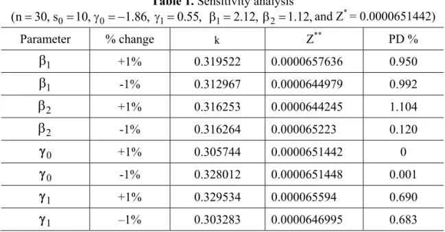
5.2 Sensitivity Analysis

To use an optimum test plan, one needs estimates of the design parameters 0

, , and

1 1 2

γ γ β

β

. These estimates sometimes may significantly affect the values of the

resulting decision variables; therefore, their incorrect choice may give a poor estimate of the quantile at design constant stress. Hence, it is important to conduct sensitivity analysis to evaluate the robustness of the resulting ALT plan.

The percentage deviations of the optimal settings are measured by

** * *

PD =(| Z −Z | / Z ) 100,× where _Z*_{is the setting obtained with the given design}

parameters, and Z is the one obtained when the parameter is mis-specified. Table 1 ** shows the optimal test plans for various deviations from the design parameter estimates. The results show that the optimal setting of Z is robust to the small deviations from baseline parameter estimates.

Table 1. Sensitivity analysis

0 0 1 1 2 (n 30, s= =10, γ = −1.86, γ =0.55, β =2.12, β =1.12,and Z* _{= 0.0000651442)} Parameter % change k Z** PD % 1

β

+1% 0.319522 0.0000657636 0.950 1

β

-1% 0.312967 0.0000644979 0.992 2

β

+1% 0.316253 0.0000644245 1.104 2

β

-1% 0.316264 0.000065223 0.120 0

γ

+1% 0.305744 0.0000651442 0 0

γ

-1% 0.328012 0.0000651448 0.001 1

γ

+1% 0.329534 0.000065594 0.690 1

γ

–1% 0.303283 0.0000646995 0.683 6. CONCLUSION

Ramp-stress ALT is characterized by stress that increases linearly with time. This paper deals with design of optimal ramp-stress ALT plan for a parallel system comprising two independent components each with Weibull lifetime. The plan is devised using masked data wherein an observation is said to be masked if the exact component that caused the system to fail is not known due to time and cost constraints. However, it can be ascertained that the cause of system failure is due to the component which belongs to some subset of the system's components. The experiment is terminated when all the test specimens put to test fail or until a pre-specified time whichever is early, i.e., the test is conducted using time-censoring (Type-I censoring) scheme. The optimal plan consists in finding optimal stress rate using D-optimality criterion that is based on minimization of

(10)

reciprocal of the determinant of Fisher information matrix. The method develop has been explained using a numerical example and sensitivity analysis carried out. The results of sensitivity analysis show that optimum plan is robust for small deviations in the true values of the model parameters.

ACKNOWLEDGMENT

The authors are grateful to the referees for their valuable comments. This research is supported by R&D Grant received from University of Delhi, Delhi, INDIA.

REFERENCES

Nelson, W. B. (1980). Accelerated Life Testing-Step-stress Models and Data Analysis,

IEEE Trans. Reliability, 29, 103-108.

Elsayed,E.A.(1996). Reliability Engineering: Addison-Wesley, Massachusets.

Bhattacharyya, G. K. and Soejoeti, Z. A. (1989). Tampered Failure Rate Model for Step-Stress Accelerated Life Test, Commun. Statist. – Theor. Meth., 18, 1627-1643.

DeGroot, M. H. andGoel, P. K. (1979). Bayesian Estimation and Optimal Designs in Partially AcceleratedLife Testing, Naval Res. Logist. Quart., 26, 223-235.

Nelson, W. (1990). Accelerated Testing: Statistical Models, Test Plans, and Data Analysis: John Wiley&Sons, New York.

Srivastava, P. W. and Gupta, T. (2015). Optimum Time-Censored Modified Ramp-Stress ALT for the Burr Type XII Distribution with Warranty: A Goal Programming Approach, International Journal of Reliability, Quality and Safety Engineering, 22, 23-23.

Usher, J. S. and Hodgson, T. J. (1998). Maximum likelihood analysis of component reliability using masked system life-data, IEEE Trans. Reliability, 37, 550-555. Escobar, L. A. and Meeker, W. Q. (1995). Planning Accelerated Life Test with two and

more experimental Factors Design for Estimation, Technometrics, 37, 411-427.

Sarhan,A. M. and Ei-Bassiouny, A. H. (2003). Estimation of component reliability in a parallel system using masked system life-data, Applied Mathematics and

(11)

Srivastava, P. W. and Savita (2016). Design of Ramp-Stress Accelerated Life Test Plans for a Parallel System with two dependent components, International Journal of

Performability Engineering, 12, 241-248.

APPENDIX

Calculations of derivatives of the log-likelihood and the elements of Fisher information matrix given in section 3.4 respectively, has been shown following.

The first partial derivatives are,

1 2 11 11 11 12 11 12 11 12 11 12 11 n n i i i i 1 11 1 1 1 1 i 1 i 1 i i i i i n 11 12 1 1 1 1 1 i i i 1 ₁₁ ₁₂ 1 1 1 t t t t L / ( 1 ( ) )Log( ) ( ) Log( ) t t t t t ( ) [ ( 1 ( ) )( ) ( ) ]Log( ) t t ( ) ( ) −β −β = = β +β −β β β β +β β = ∂ ∂β = + − + + β α α α α + − − + β + β α α α α α + β + β α α

∑

(A.1) 1 2 12 12 11 12 12 11 12 12 11 12 12 n n i i i i 2 12 1 1 1 1 i 1 i 1 i i i i i n 12 11 1 1 1 1 1 i i i 1 ₁₂ ₁₁ 1 1 1 t t t t L / ( 1 ( ) )Log( ) ( ) Log( ) t t t t t ( ) [ ( 1 ( ) )( ) ( ) ]Log( ) t t ( ) ( ) −β −β = = β +β −β β β β +β β = ∂ ∂β = + − + + β α α α α + − − + β + β α α α α α + β + β α α

∑

(A.2) ( ) ( ) ( ) 1 2 12 n n 1 1 i 2 i 3 i 4 i 5 i 6 i i 1 i 1 n 7 i 8 i 9 i 10 i i 1 L / m (t ) m (t ) m (t ) m (t ) m (t ) m (t ) m (t ) m (t ) m (t ) m (t ) = = = ∂ ∂γ = + ⋅ + + ⋅ + + + ⋅

∑

(A.3)

(

)

1 2 12 n n n 0 11 i 11 i 13 i 14 i i 1 i 1 i 1 L / m (t ) m (t ) m (t ) m (t ) = = = ∂ ∂γ =

∑

+

∑

+

∑

⋅ (A.4) The likelihood equations are obtained by setting (A.1) – (A.4) to zero. The parameter values that solve “these equations summed over all test units” are the Maximum Likelihood estimates. As the system of likelihood equations has no closed form solution in

0, ,1 1and 2,

γ γ β β therefore the maximum likelihood estimates γ γ β₀, ,₁ ₁and β₂ are obtained by maximizing (17) using NMaximize option of Mathematica 10.

1 2 12 n n n 2 2 17 i 18 i 2 1 15 i 16 i ₂ 1 i 1 i 1 i 1 19 i m (t ) (m (t )) L / m (t ) m (t ) (1 ) , (m (t )) = = = ⎛ ₋ ⎞ ∂ ∂β =⎜_⎜ + + ⎟_⎟ + γ ⎝

∑

⎠ (A.5)

(12)

56 Design of ramp-stress accelerated life test plans for a parallel system 1 2 12 12 12 12 11 12 11 12 12 11 12 12 n n 2 2 i i 2 i i 2 2 12 1 1 1 1 i 1 i 1 2 2 2 2 2 i i i i i i n 11 12 1 1 1 1 1 1 2 i i i 1 ₁₂ ₁₁ 1 1 1 t t t t L / ( ) Log( ) ( ) Log( ) t t t t t t ( ) ( ( ) 2( ) Log( )Log( ) (( ) t t (( ) ( ) ) ( 2 −β −β = = −β β + β β +β β β +β β = ⎛ ⎞ ∂ ∂β = −_β − _α _α + ⎜− _α _α ⎟ ⎝ ⎠ − − β − β α α α α α α + β + β α α − − +

∑

12 11 12 12 12 11 12 12 2 2 2 i i i i n 11 12 11 1 1 1 1 2 i i i 1 ₁₂ ₁₁ 1 1 t t t t ( ) )( ) ( ) )Log( ) , t t (( ) ( ) ) β β +β β β +β β = + β β + β α α α α β + β α α

∑

(A.6) 1 0 12 1 0 12 1 n 2 2 1 0 0 1 1 1 1 i 1 1 1 i 1 1 1 11 i 1 1 i 1 1 0 0 1 i 1 1 1 i 1 1 i 1 1 s s 1

L / (t ) (1 (1 ) log( ) log(e ( ) (1 )) log(t ) log(t )( 1 Log(t ))

1 k k

s s

1

(t ) (1 (1 ) log( ) log(e ( ) (1 )) log(t ) log(t

1 k k γ β γ − − − − = γ β γ − − − ⎛ ⎞ ∂ ∂γ = ⎜ _{+ γ} α + + γ − + γ − α − γ α − + β α ⎟ ⎝ ⎠ + α + + γ − + γ − α − γ α + γ

∑

2 12 0 12 1 12 12 11 12 11 n 1 1 1 i 1 12 i 1 i 1 2 1 0 0 1 1 2 1 n _{i 1} ₁ ₁ _{i 1} ₁ _{i 1} ₁ _{i 1} 1 i 1 1 2 i 1 1 2 1 i 1 1 i 1 )( 1 (t )) Log(t ) s s

(t ) (1 (1 ) log( ) log(e ( ) (1 )) log(t ) log(t )) ( (t )

k k ((1 )( (t ) (t ) ) (1 (t ) β − − = γ β γ β − − − − β − = β − β − ⎛ _{− + α} _{+ β} _α ⎞ ⎜ ⎟ ⎝ ⎠ α + + γ − + γ − α − γ α ⋅ −β α + + γ β α + β α + α +

∑

12 11 12 11 12 12 11 11 12 12 11 11 12 12 n 2 12 1 1 1 2 12 2 i 1 i 1 1 2 i 1 i 1 12 2 i 1 1 i 1 1 2 i 1 1 2 1 i 1 2 2 1 1 1 1 1 i 1 i 1 1 2 i 1 i 1 ) (t ) ( 1 (t ) ) 2 (t ) ( 1 (t ) ) ( (t ) ((1 )( (t ) (t ) ) (t ) * (1 (t ) ) (t ) ( 2 (t ) β β β +β β β − − − − − β − = β − β β β +β β − − − − + β α − + α + β β α − + α β β α + γ β α + β α β α + α − β β α − + α +

∑

12 11 12 n 1 i 1 1 i 1 1 2 i 1 1 2 1 i 1 )Log(t )_, ((1 )( (t ) (t ) ) − β − = β − α + γ β α + β α

∑

(A.7) 11 12 1 11 12 2 0 1 12 11 12 i i n 11 11 12 2 2 2 1 1 0 24 i 25 i 1 i 1 i i n 12 11 12 2 0 1 1 26 i 25 i 1 i 1 n 2 i 27 i 28 i 11 12 1 i 1 t t ( ) ( ) L / (m (t )(m (t )) ( ) g(t) t t ( ) ( ) s (m (t )((e ( ) (m (t )) ( ) g(t) k t (m (t )(( ) (m (t ) −β −β = −β −β γ γ = −β −β = β − β − β α α ∂ ∂γ = + ⋅ + α β − β − β α α + + ⋅ α + +β β α

∑

(m (t )) m (t ) m (t ) m (t ),29 i − 31 i 25 i + 32 i (A.8)

(13)

(

) (

)

1 2 12 12 12 12 12 12 11 11 12 11 12 n n 2 1 1 1 1 1 2 0 i 1 12 i 1 i 1 i 1 12 i 1 i 1 i 1 n 2 2 1 2 1 1 2 1 1 1 i 1 1 i 1 i 1 2 i 1 i 1 1 2 i 1 i 1 L / (t ) ( 1 Log(t ) (t ) ( 1 t ) Log(t ) (t ) ( (t ) (1 (t ) ) (t ) ( 1 (t ) ) 2 (t ) ( −β −β β − − − − − = = −β β β β β β +β − − − − − − = ∂ ∂β γ = α − + β α + α − + α + β α + α β α + α + β α − + α + β β α +

∑

12 12 11 12 11 11 12 12 12 11 12 n 2 2 1 2 1 2 1 1 1 i 1 12 2 i 1 1 i 1 i 1 1 2 i 1 i 1 n 1 1 1 1 2 i 1 i 1 2 i 1 1 i 1 i 1 1 (t ) ) ( (t ) (t ) * (1 (t ) ) (t ) ( 2 (t ) ))Log(t ) / ( (t ) (t ) ) , β β β β β +β − − − − − = β β β − − − − = − + α + β β α + β α + α − β β α + − + α α β α + β α

∑

(A.9)

(

) (

)

1 2 11 11 11 12 11 11 12 12 11 11 n n 2 1 1 1 1 1 1 0 i 1 11 i 1 i 1 i 1 11 i 1 i 1 i 1 n 2 2 1 2 1 1 2 1 1 i 1 2 i 1 i 1 1 i 1 i 1 i 1 1 2 i 1 2 i 1 L / (t ) ( 1 Log(t ) (t ) ( 1 t ) Log(t ) (t ) ( (t ) (1 (t ) ) (t ) ( 1 (t ) ) (t ) ( (t −β −β β − − − − − = = −β β β β β − − − − − = −β − − ∂ ∂β γ = α − + β α + α − + α + β α + α β α + α + β α − + α α β α +

∑

12 11 12 12 11 12 11 12 11 12 11 12 11 12 n 12 1 2 12 1 i 1 1 i 1 i 1 1 1 2 i 1 1 i 1 2 i 1 n 1 1 1 1 2 i 1 i 1 i 1 1 1 2 i 1 1 i 1 2 i 1 2 2 1 2 11 1 i 1 2 ) (1 (t ) ) (t ) ( 1 (t ) ) ( (t ) (t ) ) 2 (t ) ( 1 (t ) )Log(t ) ( (t ) (t ) ) ( (t ) ( β − β − β − β β β − − = β +β β − − − β β − − = β − + α + β α − + α β α + β α β β α − + α α + β α + β α β β α + β +

∑

12 11 12 11 12 11 12 11 n 12 1 1 1 1 i 1 i 1 1 2 i 1 i 1 i 1 1 1 2 i 1 1 i 1 2 i 1 t ) (1 (t ) ) (t ) ( 2 (t ) ))Log(t ) , ( (t ) (t ) ) β β β +β β − − − − − β β − − = α + α − β β α − + α α β α + β α

∑

(A.10) 1 0 12 1 0 12 1 n 2 1 0 0 1 1 1 2 1 i 1 1 1 i 1 1 1 11 i 1 1 i 1 1 0 0 1 i 1 1 1 i 1 1 i 1 1 s s 1

1 k k

s s

1

(t ) (1 (1 ) log( ) log(e ( ) (1 )) log(t ) log(t

1 k k γ β γ − − − − = γ β γ − − ⎛ ⎞ ∂ ∂β γ = ⎜ _{+ γ} α + + γ − + γ − α − γ α − + β α ⎟ ⎝ ⎠ + α + + γ − + γ − α − γ α + γ

∑

2 12 0 12 1 12 12 11 12 1 n 1 1 1 i 1 12 i 1 i 1 2 1 0 0 1 1 2 1 n _{i 1} ₁ ₁ _{i 1} ₁ _{i 1} ₁ _{i 1} 1 i 1 1 2 i 1 1 2 1 i 1 1 i 1 )( 1 (t )) Log(t ) s s

k k ((1 )( (t ) (t ) ) (1 (t ) β − − − = γ β γ β − − − − β − = β − β − ⎛ _{− + α} _{+ β} _α ⎞ ⎜ ⎟ ⎝ ⎠ α + + γ − + γ − α − γ α ⋅ −β α + + γ β α + β α + α +

∑

12 1 11 12 11 12 12 11 11 12 12 11 11 12 1 n 2 12 1 1 1 2 12 2 i 1 i 1 1 2 i 1 i 1 12 2 i 1 1 i 1 1 2 i 1 1 2 1 i 1 2 2 1 1 1 1 1 i 1 i 1 1 2 i 1 i 1 ) (t ) ( 1 (t ) ) 2 (t ) ( 1 (t ) ) ( (t ) ((1 )( (t ) (t ) ) (t ) * (1 (t ) ) (t ) ( 2 (t ) β β β +β β β − − − − − β − = β − β β β +β β − − − − + β α − + α + β β α − + α β β α + γ β α + β α β α + α − β β α − + α +

∑

12 2 11 12 n 1 i 1 1 i 1 1 2 i 1 1 2 1 i 1 )Log(t )_, ((1 )( (t ) (t ) ) − β − = β − α + γ β α + β α

∑

(A.11)

(14)

58 Design of ramp-stress accelerated life test plans for a parallel system 1 0 11 1 0 11 1 n 2 1 0 0 1 1 1 1 1 i 1 1 1 i 1 1 i 1 12 i 1 1 i 1 1 0 0 1 i 1 1 1 i 1 1 i 1 s s 1

1 k k

s s

1 _(t ₎ _{(1 (1} _{) log( ) log(e ( ) (1} _{)) log(t} ₎ _log(t

1 k k γ β γ − − − − = γ β γ − − ⎛ ⎞ ∂ ∂β γ = _⎜ α + + γ − + γ − α − γ α − + β α _⎟ + γ ⎝ ⎠ + α + + γ − + γ − α − γ α + γ

∑

2 11 0 11 1 12 12 11 11 12 n 1 1 1 1 i 1 11 i 1 i 1 1 0 0 1 1 n _{i 1} ₁ ₁ _{i 1} ₁ _{i 1} 1 1 2 i 1 1 1 i 1 2 i 1 1 1 2 i 1 i 1 )( 1 (t )) Log(t ) s s

(t ) (1 (1 ) log( ) log(e ( ) (1 )) log(t ) log(t ))

k k ((1 )( (t ) (t ) ) 2 (t ) ( 1 (t β − − − = γ β γ − − − β β − − = β +β − − ⎛ _{− + α} _{+ β} _α ⎞ ⎜ ⎟ ⎝ ⎠ α + + γ − + γ − α − γ α + + γ β α + β α β β α − + α +

∑

12 11 12 11 12 12 11 11 12 11 12 11 n 1 2 12 2 12 1 11 1 i 1 2 i 1 i 1 1 1 2 i 1 1 1 i 1 2 i 1 1 1 1 1 1 2 1 2 i 1 i 1 i 1 1 1 i 1 2 i 1 1 1 i ) ) ( (t ) (t ) *(1 (t ) ) ((1 )( (t ) (t ) ) (t ) ( 2 (t ) )Log(t t ) / ((1 )( (t ) (t ) ) ((1 )( (t β − β − β − β β β − − = β +β β β β − − − − − β β α +β α + α + γ β α + β α β β α − + α α + γ β α + β α − + γ β

∑

12 12 11 n 1 1 2 i 1 1 2 i 1 , )β (t )β ) − − = α + β α

∑

(A.12) 11 12 12 11 1 0 1 11 12 12 ( ) 1 2 1 2 1 0 i 1 1 i 1 2 1 1 n 2 1 0 1 1 1 i 1 0 1 i 1 1 i 1 ( ) 1 2 1 2 1 i 1 1 i 1 2 i 1 1 s 1 (t ) ( (t ) (t ) )(1 (1 )log( ) 1 k L / s

log(e ( ) (1 )) log(t ) log(t ) k 1 _(t ₎ _{( (t} ₎ _(t ₎ 1 − β +β β β − − − γ γ − − = − β +β β β − − − − ⎛ _α _β _α _{+β α} _{+ + γ} ⎞ ⎜ _{+ γ} ⎟ ⎜ ⎟ ∂ ∂γ γ = ⎜ ⎟ − + γ − α − γ α ⎜ ⎟ ⎝ ⎠ − α β α +β α + γ +

∑

(

)

11 2 0 1 12 12 11 0 1 n 1 1 i 1 0 1 i 1 1 i 1 n 1 1 2 20 i 21 i 22 i 23 i 1 1 i 1 2 i 1 i 1 s )(1 (1 )log( ) k s

log(e ( ) (1 )) log(t ) log(t ) k m (t )(m (t )(m (t ) m (t ))) / ((1 )( (t ) (t ) ) ) , γ γ − − = β β − − = ⎛ _{+ + γ} ⎞ ⎜ ⎟ ⎜ ⎟ ⎜ ⎟ − + γ − α − γ α ⎜ ⎟ ⎝ ⎠ + + γ β α + β α

∑

(A.13) 11 12 11 12 12 12 11 2 i i i n 11 12 2 1 1 1 1 2 2 i i i 1 ₁ ₂ 1 1 t t t ( ( ) ( 1 ( ) )( 1 ( ) )) L / t t ( ( ) ( ) ) β + β β β β β = − − + β − + β α α α ∂ ∂β β = β + β α α

∑

(A.14) The elements of the Fisher information matrix for an observation are the negative expectations of these second partial derivatives:

2 2 17 i 18 i 2

1 1 ₀ 15 i 2 ₀ 16 i 12 ₀ ₂ 1

19 i

m (t ) (m (t )) E[ L / ] E[n ] m (t ) E[n ] m (t ) E[n ] (1 ) ,

(m (t ))

∞ ∞ ∞

⎛ ₋ ⎞

∂ ∂β = ⎜_⎜ + + ⎟_⎟ + γ

(15)

P. W. Srivastava, Savita 59 12 12 12 12 11 12 11 12 11 12 12 2 2 i i 2 i i 2 2 1 ₀ 2 ₀ 12 1 1 1 1 2 2 2 2 2 i i i i i i 11 12 1 1 1 1 1 1 12 2 i i 12 11 1 1 1 t t t t

E[ L / ] E[n ] ( ) Log( ) E[n ] ( ) Log( )

t t t t t t ( ) ( ( ) 2( ) Log( )Log( ) (( ) E[n ] _t _t (( ) ( ) ) ∞ _−β ∞ _−β −β β + β β +β β β +β β ⎛ ⎞ ∂ ∂β = − − + _⎜− _⎟ β α α _⎝ α α _⎠ − − β − β α α α α α α β + β α α

∫

12 11 12 12 11 12 12 0 2 2 2 i i i i 11 12 11 1 1 1 1 12 0 _i _i ₂ 12 11 1 1 t t t t ( 2 ( ) )( ) ( ) )Log( ) E[n ] _t _t , (( ) ( ) ) ∞ β β +β β ∞ β +β β − − + β β + β α α α α β + β α α

∫

(A.16) 11 12 1 11 12 0 1 11 12 i i n 11 11 12 2 2 2 1 1 0 1 ₀ 24 i 25 i i 1 i 1 i i 12 11 12 2 0 1 1 2 ₀ 26 i 25 i i 1 i 12 27 i 1 t t ( ) ( ) E[ L / ] E[n ] (m (t )(m (t )) ( ) g(t)dt t t ( ) ( ) s E[n ] (m (t )e ( ) (m (t )) ( ) g(t)dt k t E[n ] (m (t )(( ) ( −β −β ∞ = −β −β ∞ _γ _γ −β −β β − β − β α α ∂ ∂γ = + ⋅ α β − β − β α α + + ⋅ α + α

∑

∫

12 n 2 28 i 11 12 29 i 31 i 25 i 32 i i 0 i 1 m (t ) (m (t )) m (t ) m (t ) m (t )dt , ∞ = +β β − +

∑

∫

(A.17)

(

)

12 12 12 12 12 11 11 12 11 2 1 1 1 1 1 2 0 1 ₀ i 1 12 i 1 2 ₀ i 1 i 1 12 i 1 2 2 1 2 1 1 2 1 1 1 12 i 1 1 i 1 i 1 2 i 1 i 1 1 2 i 1

E[ L / ] E[n ] (t ) ( 1 Log(t ) E[n ] (t ) ( 1 t ) Log(t ) E[n ] t ) ( (t ) (1 (t ) ) (t ) ( 1 (t ) ) 2 (t ) ∞ ₋ _−β ₋ ∞ ₋ _−β ₋ _β ₋ −β β β β β β + − − − − − − ∂ ∂β γ = α − + β α + α − + α + β α + α β α + α + β α − + α + β β α

∫

12 12 11 12 11 11 12 12 11 12 0 2 2 1 2 1 2 1 1 1 12 ₀ i 1 12 2 i 1 1 i 1 i 1 1 2 i 1 1 1 1 1 2 12 ₀ i 1 i 1 2 i 1 1 i 1 E[n ] ( 1 (t ) ) ( (t ) (t ) * (1 (t ) ) (t ) E[n ] ( 2 (t ) ))Log(t ) / ( (t ) (t ) ) , ∞ _β ∞ ₋ _β ₋ _β ₋ _β ₋ _β ₋ _{β +β} ∞ ₋ _β ₋ ₋ _β ₋ _β + − + α + β β α + β α + α − β β α + − + α α β α + β α

∫

(A.18)

(

)

2

(

)

11 11 11 11 11 12 12 11 n 2 1 1 1 1 1 1 0 1 ₀ i 1 11 i 1 2 ₀ i 1 i 1 11 i 1 i 1 2 2 1 2 1 1 2 1 1 12 ₀ i 1 2 i 1 i 1 1 i 1 i 1 12

E[ L / ] E[n ] (t ) ( 1 Log(t ) E[n ] (t ) ( 1 t ) Log(t ) E[n ] (t ) ( (t ) (1 (t ) ) (t ) ( 1 (t ) ) ( E[n ] ∞ ₋ _−β ₋ ∞ ₋ _−β ₋ _β ₋ = ∞ ₋ _−β ₋ _β ₋ _β ₋ _β ₋ _β ∂ ∂β γ = α − + β α + α − + α + β α + α β α + α + β α − + α +

∑

∫

11 11 12 12 11 12 11 11 12 11 12 11 2 2 1 2 1 1 2 1 1 i 1 2 i 1 i 1 1 i 1 i 1 1 1 2 0 1 i 1 2 i 1 1 1 1 1 2 i 1 i 1 i 1 12 ₀ ₁ ₁ ₂ 1 i 1 2 i 1 12 t ) ( (t ) (1 (t ) ) (t ) ( 1 (t ) ) ( (t ) (t ) ) 2 (t ) ( 1 (t ) )Log(t ) E[n ] ( (t ) (t ) ) E[n −β β β β β − − − − − ∞ β β − − β +β β − − − ∞ β β − − α β α + α + β α − + α β α + β α β β α − + α α + β α + β α +

∫

12 11 12 11 12 11 12 11 2 2 2 1 2 1 1 1 1 1 11 1 i 1 2 i 1 i 1 1 2 i 1 i 1 i 1 1 1 2 0 1 i 1 2 i 1 ( (t ) (t ) (1 (t ) ) (t ) ( 2 (t ) ))Log(t ) ] , ( (t ) (t ) ) β β β β +β β − − − − − − ∞ β β − − β β α + β α + α − β β α − + α α β α + β α

∫

(A.19)

(16)

60 Design of ramp-stress accelerated life test plans for a parallel system 0 12 1 0 12 1 2 1 0 0 1 1 1 2 1 1 ₀ i 1 1 1 i 1 1 1 11 i 1 i 1 1 0 0 2 i 1 1 1 i 1 1 s s 1

E[ L / ] E[n ] (t ) (1 (1 ) log( ) log(e ( ) (1 )) log(t ) log(t )( 1 Log(t )) dt

1 k k

s s

1

E[n ] (t ) (1 (1 ) log( ) log(e ( ) (1 )) log(t

1 k k ∞ ₋ _β _γ _γ ₋ ₋ ₋ γ β γ − − ⎛ ⎞ ∂ ∂β γ = ⎜ _{+ γ} α + + γ − + γ − α − γ α − + β α ⎟ ⎝ ⎠ + α + + γ − + γ − α + γ

∫

12 0 12 1 12 11 12 1 1 1 1 1 i 1 i 1 12 i 1 i 0 2 1 0 0 1 1 2 1 i 1 1 1 i 1 1 i 1 1 i 1 12 ₁ 1 2 i 1 1 2 1 i 1 ) log(t )( 1 (t )) Log(t ) dt s s

k k E[n ] dt ((1 )( (t ) (t ) ) ∞ ₋ ₋ _β ₋ γ β γ β − − − − β − β − ⎛ ⎞ − γ α − + α + β α ⎜ ⎟ ⎝ ⎠ α + + γ − + γ − α − γ α ⋅ −β α + + γ β α + β α

∫

11 11 12 11 12 12 11 11 12 12 11 i 0 2 2 1 2 1 1 1 1 2 1 i 1 2 i 1 i 1 1 2 i 1 i 1 12 2 i 1 12 0 1 i 1 2 i 1 1 2 1 i 1 2 2 1 1 1 i 1 i 1 1 2 12 (1 (t ) ) (t ) ( 1 (t ) ) 2 (t ) ( 1 (t ) ) ( (t ) E[n ] dt ((1 )( (t ) (t ) ) (t ) *(1 (t ) ) E[n ] ∞ β β β β +β β β − − − − − − ∞ β − β − β β − − + α + β α − + α + β β α − + α β β α + + γ β α + β α β α + α − β β +

∫

11 12 12 11 12 1 1 1 i 1 i 1 i 1 i 1 0 1 2 i 1 1 2 1 i 1 (t ) ( 2 (t ) )Log(t ) dt , ((1 )( (t ) (t ) ) β +β β − − − ∞ β − β − α − + α α + γ β α + β α

∫

(A.20) 0 11 1 0 11 1 2 1 0 0 1 1 1 1 1 1 ₀ i 1 1 1 i 1 1 i 1 12 i 1 i 1 1 0 0 2 i 1 1 1 i 1 1 s s 1

1 k k

s s

1

E[n ] (t ) (1 (1 ) log( ) log(e ( ) (1 )) log(t

1 k k ∞ ₋ _β _γ _γ ₋ ₋ ₋ γ β γ − ⎛ ⎞ ∂ ∂β γ = ⎜ _{+ γ} α + + γ − + γ − α − γ α − + β α ⎟ ⎝ ⎠ + α + + γ − + γ − α + γ

∫

11 0 11 1 12 11 1 1 1 1 1 i 1 i 1 11 i 1 i 0 1 0 0 1 1 i 1 1 1 i 1 1 i 1 12 0 1 1 2 i 1 1 i 1 2 i 1 1 2 12 ) log(t )( 1 (t )) Log(t ) dt s s

(t ) (1 (1 ) log( ) log(e ( ) (1 )) log(t ) log(t ))

k k E[n ] dt ((1 )( (t ) (t ) ) 2 ( E[n ] ∞ ₋ ₋ ₋ _β ₋ γ β γ − − − ∞ β β − − ⎛ _{− γ} _α _{− + α} _{+ β} _α ⎞ ⎜ ⎟ ⎝ ⎠ α + + γ − + γ − α − γ α + + γ β α + β α β β +

∫

11 12 11 12 11 12 12 11 11 12 11 12 2 2 1 1 2 1 2 1 1 i 1 i 1 11 1 i 1 2 i 1 i 1 i 1 1 2 0 1 1 i 1 2 i 1 1 1 1 1 1 2 i 1 i 1 i 1 1 1 i 1 12 t ) ( 1 (t ) ) ( (t ) (t ) *(1 (t ) ) dt ((1 )( (t ) (t ) ) (t ) ( 2 (t ) )Log(t t ) / ((1 )( (t ) E[n ] β +β β β β β − − − − − ∞ β β − − β +β β β − − − − α − + α β β α +β α + α + γ β α + β α β β α − + α α + γ β α −

∫

11 12 11 1 2 2 i 1 i 1 1 2 0 1 1 i 1 2 i 1 (t ) ) _{dt ,} ((1 )( (t ) (t ) ) β − ∞ β β − − + β α + γ β α + β α

∫

(A.21) 11 12 12 11 0 1 11 12 12 ( ) 1 2 1 2 1 0 i 1 1 i 1 2 1 1 2 1 0 1 1 ₀ i 1 1 0 1 i 1 1 i 1 ( ) 1 2 1 i 1 1 i 1 1 2 s 1 _(t ₎ _{( (t} ₎ _(t ₎ _{)(1 (1} _{)log( )} 1 k E[ L / ] E[n ] dt s

log(e ( ) (1 )) log(t ) log(t ) k 1 (t ) ( (t ) 1 E[n ] − β +β β β − − − ∞ γ γ − − − β +β β − − − ⎛ _α _β _α _{+β α} _{+ + γ} ⎞ ⎜ _{+ γ} ⎟ ⎜ ⎟ ∂ ∂γ γ = ⎜ ⎟ − + γ − α − γ α ⎜ ⎟ ⎝ ⎠ − _α _β _α + γ +

∫

(

)

11 0 1 12 11 2 1 0 2 i 1 1 i 0 1 1 0 1 i 1 1 i 1 1 1 2 12 ₀ 20 i 21 i 22 i 23 i 1 1 i 1 2 i 1 i s (t ) )(1 (1 )log( ) k _dt s

log(e ( ) (1 )) log(t ) log(t ) k E[n ] m (t )(m (t )(m (t ) m (t ))) / ((1 )( (t ) (t ) ) ) dt , β − ∞ γ γ − − ∞ ₋ _β ₋ _β ⎛ _+β _α _{+ + γ} ⎞ ⎜ ⎟ ⎜ ⎟ ⎜ ⎟ − + γ − α − γ α ⎜ ⎟ ⎝ ⎠ + + γ β α + β α

∫

(A.22)

(17)

P. W. Srivastava, Savita 61 11 12 11 12 12 11 2 i i i 11 12 2 1 1 1 1 2 12 ₀ i 2 i i 1 2 1 1 t t t ( ( ) ( 1 ( ) )( 1 ( ) )) E[ L / ] E[n ] dt , t t ( ( ) ( ) ) β + β β β ∞ β β − − + β − + β α α α ∂ ∂β β = β + β α α

∫

(A.23) 0 12 1 0 12 1 2 2 1 0 0 1 1 1 1 1 ₀ i 1 1 1 i 1 1 1 11 i 1 i 1 1 0 0 1 2 i 1 1 1 i 1 1 s s 1

1 k k

s s

1

E[n ] (t ) (1 (1 ) log( ) log(e ( ) (1 )) log(t

1 k k ∞ ₋ _β _γ _γ ₋ ₋ ₋ γ β γ − − ⎛ ⎞ ∂ ∂γ = ⎜ _{+ γ} α + + γ − + γ − α − γ α − + β α ⎟ ⎝ ⎠ + α + + γ − + γ − α + γ

∫

12 0 12 1 12 11 12 1 1 1 1 i 1 i 1 12 i 1 i 0 2 1 0 0 1 1 2 1 i 1 1 1 i 1 1 i 1 1 i 1 12 1 i 1 2 i 1 1 2 1 i 1 ) log(t )( 1 (t )) Log(t ) dt s s

k k E[n ] dt ((1 )( (t ) (t ) ) ∞ ₋ ₋ _β ₋ γ β γ β − − − − β − β − ⎛ _{− γ} _α _{− + α} _{+ β} _α ⎞ ⎜ ⎟ ⎝ ⎠ α + + γ − + γ − α − γ α ⋅ −β α + + γ β α + β α

∫

11 11 12 11 12 12 11 11 12 12 11 0 2 2 1 2 1 1 1 1 2 1 i 1 2 i 1 i 1 1 2 i 1 i 1 12 2 i 1 12 ₀ ₁ i 1 2 i 1 1 2 1 i 1 2 2 1 1 1 i 1 i 1 1 2 12 (1 (t ) ) (t ) ( 1 (t ) ) 2 (t ) ( 1 (t ) ) ( (t ) E[n ] dt ((1 )( (t ) (t ) ) (t ) *(1 (t ) ) ( E[n ] ∞ β β β β +β β β − − − − − − ∞ β − β − β β − − + α + β α − + α + β β α − + α β β α + + γ β α + β α β α + α − β β +

∫

11 12 12 11 12 1 1 1 i 1 i 1 i 1 i 1 0 1 2 i 1 1 2 1 i 1 t ) ( 2 (t ) )Log(t )_{dt ,} ((1 )( (t ) (t ) ) β +β β − − − ∞ β − β − α − + α α + γ β α + β α

∫

(A.24)

(18)

62 Design of ramp-stress accelerated life test plans for a parallel system 11 12 11 12 0 1 1 0 1 i i i i 1 i 1 2 11 1 1 1 1 i i ₁ 11 11 12 (1 ) 0 1 1 2 i 1 1 0 0 3 i 1 1 i 4 i 1 1 t t t t

where : m (t ) ( ( 1 ( ) )Log( )) (( ) Log( )) ,

t t ( ) ( ) s m (t ) ( ) (e ( ) (1 )) k s s m (t ) (1+(1 )Log( ) Log(e ( ) (1 ))), k k t m (t ) (( −β −β −β −β γ γ +γ γ γ = + − + β + β β α α α α β − β − β α α = × + γ α = + γ + + γ = α 11 12 11 12 0 1 1 0 1 11 12 i i i 1 2 1 12 1 1 i i ₁ 12 11 12 (1 ) 0 1 1 5 i 1 1 0 0 6 i 1 1 i i 1 1 7 i t 1 t t ) Log( )) ( ( 1 ( ) )Log( )) , t t ( ) ( ) s m (t ) ( )(e ( ) (1 )) , k s s m (t ) (1+(1 )Log( ) Log(e ( ) (1 ))), k k t t ( ) ( ( 1 ( m (t ) −β −β −β −β γ γ +γ γ γ β +β β + + − + β α β α α β − β − β α α = + γ α = + γ + + γ + − − + α α = 11 12 11 11 12 11 11 12 12 11 12 11 12 12 1 i i i 11 12 1 1 1 1 2 i i 11 12 1 1 i i i i i 12 11 1 1 1 1 1 8 i 2 2 i i 12 11 1 1 i 1 9 i t t t ) )( ) ( ) )Log( ) , t t ( ) ( ) t t t t t ( ) ( ( 1 ( ) )( ) ( ) )Log( ) m (t ) _t _t , ( ) ( ) t ( 1 ( ) m (t ) −β β β β +β β β +β −β β β β +β β −β β + β α α α _β β + β α α + − − + β + β α α α α α = β β + β α α − + α = 1 11 12 12 11 12 12 11 0 1 1 0 1 11 12 2 2 i i i 11 11 12 12 1 1 1 1 11 12 1 1 1 (1 ) 0 0 0 10 i 1 1 1 i i 11 11 1 1 1 11 i t t t )( ) 2 ( 1 ( ) )( ) , t t ( ) ( ) s s s m (t ) (e ( ) (1 )) (1+(1 )Log( ) Log(e ( ) (1 ))) k k k t t ( ) ( ) m (t ) ( β +β −β β −β β β γ γ +γ γ γ −β −β β − β β + − + β α α α α β + β α α = + γ ⋅ + γ + + γ β − β − β α α = 0 1 0 1 1 11 12 0 1 0 1 1 11 11 12 12 11 1 1 2 1 1 0 0 1 1 i i ₁ 12 11 12 1 1 0 0 1 1 12 i 1 1 2 i i i i 11 11 12 1 1 1 1 13 i s s )(e ( ) (e ( ) (1 )) , k k t t ( ) ( ) s s m (t ) ( )(e ( ) (e ( ) (1 )) , k k t t t t ( 1 ( ) )( ) 2 ( 1 ( ) )( ) m (t ) ( − + γ γ γ γ +γ −β −β − + γ γ γ γ +γ −β −β +β β β −β + γ α β − β − β α α = + γ α − + β − β β + − + α α α α = 2 12 11 0 1 0 1 1 11 11 2 12 i i 1 11 12 1 1 1 1 1 2 0 0 i i 14 i 1 15 i 11 1 1 2 i i 16 i 1 1 ), t t (( ) ( ) ) s s 1 t t m (t ) (e ( ) (e ( ) (1 )) ,m (t ) ( ) Log( ) , k k t t m (t ) ( ) Log( ) , β β − + γ γ γ γ +γ −β −β β α β + β α α = + γ = − − β α α = − α α

(19)

P. W. Srivastava, Savita 63 11 11 12 11 12 11 11 11 12 11 11 12 11 2 2 i i i i 17 i 12 1 1 1 1 2 2 2 2 2 i i i i i 18 i 11 11 12 12 1 1 1 1 1 i i 19 i 11 12 1 1 1 20 i i 1 t t t t m (t ) ( ) ( ( ) 2( ) Log( ), t t t t t m (t ) ( ) ( 2 ( ) )( ) ( ) )Log( ) , t t m (t ) ( ) ( ) , m (t ) (t ) −β β + β β +β β β β +β β β +β β − = − − β α α α α = β − − + β β + β α α α α α = β + β α α = α 11 12 11 12 11 12 11 12 11 12 11 12 11 12 11 ( ) 4 13 4 13 2 2 21 i 2 i 1 1 i 1 1 2 2( ) 2( ) ( 2 ) ( 2 ) 1 1 1 3 1 22 i i 1 i 1 i 1 1 2 i 1 ( 2 ) 1 3 1 23 i i 1 2 1 i 1 ,m (t ) (t ) (t ) , m (t ) 2(t ) (t ) (t ) (t ) , m (t ) ( 2 (t ) ) (t ) ( 2 − β +β − β − β β +β β +β β + β β + β − − − − β β + β − − = β α +β α + β β = α + α + α − β β α = − + α − β β α − + 12 0 1 11 11 12 0 1 0 1 1 1 0 0 i 1 1 1 1 1 i 1 1 i 1 2 i i i 11 11 11 12 12 1 1 1 24 i ₂ 1 1 1 1 0 0 25 i 1 26 i s s (t ) ))(1 (1 )log( ) log(e ( ) (1 )) k k log(t ) log(t ), t t t ( ) ( ) ( ) ( 1 ) m (t ) , s s m (t ) (e ( ) (e ( ) (1 )) , k k m (t ) γ β γ − − − −β −β −β − + γ γ γ γ +γ α + + γ − + γ − α − γ α β − β + β + − + β β α α α = α = + γ − = 11 11 12 12 11 12 12 11 12 11 12 12 2 i i i i 11 11 12 12 12 1 1 1 1 2 1 i 27 i 2 i i 2 1 1 11 12 1 1 3 4 3 3 i i i i 28 i 11 12 12 29 i 1 1 1 1 t t t t ( ) ( ) ( ) ( 1 ( ) ) , 1 t m (t ) _t _t (( ) , (( ) ( ) ) t t t t m (t ) ( ) ( ) ( 1 ( ) ),m (t ) 3 ( ) −β −β −β β −β −β β β − β β β β β + β + β − + + β β α α α α α = α α β + β α α = β − β − + + β = − + α α α α 12 12 12 11 12 11 12 11 12 12 11 12 11 11 i 12 1 i i i i i 30 i 12 1 1 1 1 1 2 2 3 i i i i i i 31 i 12 11 11 12 1 1 1 1 1 1 32 i t ( 2 ( ) , t t t t t m (t ) (3 ( ) )( ) (( ) ( ) 2( ) ) , t t t t t t m (t ) ( ) (( ( ) ( ( 1 ( ) )( ) ( 2 ( ) )( ) )))), ( m (t ) ( β β β β β β +β β +β β β β β β − + β α = − + + + β α α α α α = β β + β − − + − + β α α α α α α − = 11 11 12 12 11 12 12 11 2 2 i i i i 11 11 12 12 1 1 1 1 i i 1 11 12 1 1 t t t t 1 ( ) )( ) 2 ( 1 ( ) )( ) )(g(t)), t t (( ) ( ) ) −β −β +β β β −β β β + β − β β + − + β α α α α α β + β α α