이용자는 아래의 조건을 따르는 경우에 한하여 자유롭게 l 이 저작물을 복제, 배포, 전송, 전시, 공연 및 방송할 수 있습니다. 다음과 같은 조건을 따라야 합니다: l 귀하는, 이 저작물의 재이용이나 배포의 경우, 이 저작물에 적용된 이용허락조건 을 명확하게 나타내어야 합니다. l 저작권자로부터 별도의 허가를 받으면 이러한 조건들은 적용되지 않습니다. 저작권법에 따른 이용자의 권리는 위의 내용에 의하여 영향을 받지 않습니다. 이것은 이용허락규약(Legal Code)을 이해하기 쉽게 요약한 것입니다. Disclaimer 저작자표시. 귀하는 원저작자를 표시하여야 합니다. 비영리. 귀하는 이 저작물을 영리 목적으로 이용할 수 없습니다. 변경금지. 귀하는 이 저작물을 개작, 변형 또는 가공할 수 없습니다.
A study on the performance of a cross-flow
air turbine utilizing an orifice for OWC
wave energy converters
Supervisor Prof. Young-Ho LEE, Ph.D
February 2017
Department of Mechanical Engineering
Graduate School of Korea Maritime and Ocean University
Contents
List of Tables ... iii
List Figures ... iv
Abstract ... vii
Nomenclature ... ix
Chapter 1. Introduction ... 1
1.1 Background ... 1
1.2 Wave Energy Converter ... 2
1.3 Literature Survey ... 4
1.3.1 OWC ... 4
1.3.2 Air turbine for OWC WEC ... 5
1.3.3 Linear wave theory ... 7
1.4 Objective of research ... 12
Chapter 2. CFD analysis of a cross-flow air turbine 14
2.1 ANSYS CFD Code ... 14
2.1.1 Discretization of the governing equations ... 14
2.1.2 Turbulence model ... 16
2.2 Design of cross-flow turbine ... 19
2.3 Steady State simulation ... 20
2.3.1 Numerical analysis setup ... 21
2.4 Transient simulation ... 28
2.4.1 Numerical setup ... 29
2.4.2 Data analysis ... 30
2.4.3 CFD result and discussion... 35
Chapter 3. Validation of an Orifice for turbine damping effects ... 47
3.1 Ideal Air ... 47
3.2 Orifice PTO system ... 48
3.3 Design of Orifice ... 49
3.4 Numerical analysis of Orifice ... 50
3.4.1 Numerical analysis setup ... 50
3.4.2 CFD result and discussion... 52
3.5 Experimental analysis of Orifice ... 55
3.6 Result of experiment and comparative study ... 58
Chapter 4. Conclusion... 62
Acknowledgements... 64
List of Tables
Table 1 Worldwide wave power installed capacity [4]... 2
Table 2 Selection of WEC Device developers [5] ... 3
Table 3 Summary of linear (Airy) wave theory characteristics [21] ... 12
Table 4 Overview of turbulent flow simulation methods [22] ... 17
Table 5 Design parameters for the cross-flow air turbine ... 20
Table 6 Boundary condition of CFX pre setup for the cross-flow air turbine in steady state simulation ... 23
Table 7 Boundary condition of CFX pre setup for the cross-flow air turbine in transient simulation ... 30
Table 8 Summary of performance of the model scaled cross-flow air turbine by CFD ... 46
List Figures
Figure 1 Oscillating water column WEC [7] ... 4
Figure 2 Definition sketch for dimensional linear wave theory (LWT) boundary
value [19] ... 8
Figure 3 Nomenclature of a linear water wave, having a sinusoidal profile [20] ... 10
Figure 4 Properties of waves under several depth conditions: (a) deep water, (b)
intermediate water, (c) shallow water [20] ... 11
Figure 5 Configuration of control volume definition (a) and mesh element (b) [22]
... 14
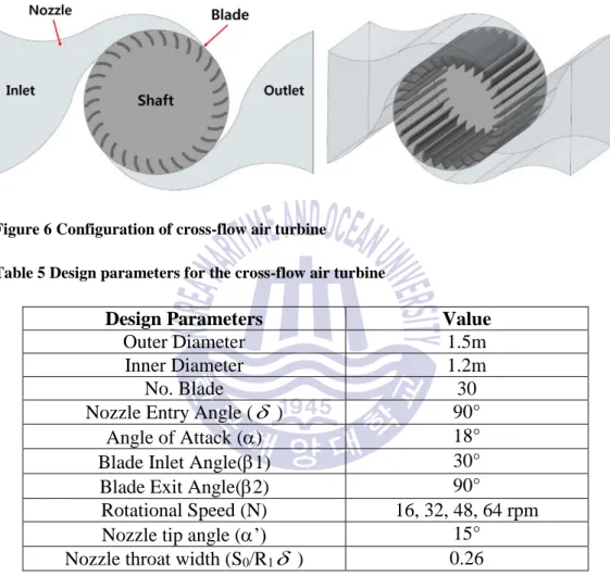
Figure 6 Configuration of cross-flow air turbine ... 20
Figure 7 Meshing of the cross-flow air turbine by ICEM CFD ... 22
Figure 8 Configuration of CFX pre setup domain for the cross-flow air turbine in
steady state ... 22
Figure 9 Schematic configuration of the cross-flow air turbine with division of runner
flow passage ... 24
Figure 10 Velocity vectors in the flow field of the turbine domain at 32rpm rotational
Figure 14 Visual configuration of the division of time series data into segments for
phase averaging [25] ... 31
Figure 15 Representation of times series cycles for (a) pressure gap between
upstream and downstream and (b) flow rate through the turbine in one segment by
phase averaging (T=1.5sec) ... 33
Figure 16 Phase-averaged profile of (a) pressure gap and (b) flow rate (T=1.25sec)
... 34
Figure 17 Velocity vectors in the flow field of the turbine domain at 1000rpm
rotational speed and 2 sec period ... 36
Figure 18 Pressure contours in the flow field of the turbine domain at 1000rpm
rotational speed and 2 sec period ... 37
Figure 19 Power distribution on entire rotor at different wave periods ... 40
Figure 20 Pressure against flow rate with phase averaging at 1000rpm rotational
speed... 42
Figure 21 Representation of phase averaged times series cycles for turbine torque in
one segment... 44
Figure 22 Phase averaged shaft power and air power ... 46
Figure 23 Meshing of the orifice plate by ICEM CFD ... 51
Figure 24 Configuration of CFX pre setup domain for the orifice plate in transient
simulation ... 51
Figure 25 Phase averaged pressure drop and flow rate diagram of the orifice plates
with the turbine result ... 54
Figure 28 Experimental setup with OWC chamber in wave tank... 57
Figure 29 Experimental equipment in OWC chamber for measurement ... 58
Figure 30 Validations of orifice plate as substitute for the cross-flow air turbine
A study on the performance of a cross-flow air turbine
utilizing an orifice for OWC wave energy converters
Hong Goo Kang
Department of Mechanical Engineering
Graduate School of Korea Maritime and Ocean University
Abstract
Ocean energy which includes tidal energy, ocean thermal energy conversion, wave energy and other marine energy currents, hold an enormous amount of untapped energy that, if exploited extensively, have a potential for contributing significantly to the electricity supply of countries facing the sea. One of the most successful and most extensively investigated devices for extracting wave energy is the Oscillating Water Column (OWC). OWCs have been widely developed due to its potential deployment if various water conditions and its simplicity in design. The common OWC wave energy converter consists of fixed or floating structure, which opens to the sea below the water surface and absorbs wave energy, and a turbine coupled to a generator. Wave motion inside the chamber induces an exhalation and inhalation of the trapped air which drive the bi-directional turbine at the opening of the device. The turbine is connected to a generator so that mechanical motion from the rotating blade is converted to an electrical energy.
A cross-flow air turbine is a candidate for use of a self-starting turbine due to its characteristic, high coefficient at a low tip speed ratio. In addition, it has excellent stability
and low noise. With its characteristics this turbine may be more suitable at places where require low noise compared to typical commercialized air turbines such as Wells and impulse turbine. In this research, the investigation of cross-flow air turbine for OWC wave energy converter have been undertaken. First, a numerical analysis of the turbine by CFD have been conducted in order to acquire its performance characteristics in various range of the flow rate with different rotational speed of the rotor. Model scale analysis was proposed to design and compare with experimental model, and 1/16 model scale was determined. In addition, the orifice plate as substitute was adopted not only to simulate the behavior of the turbine by numerical analysis and experiment but also to verify the CFD result with the experiment result. The size of the orifice plate was determined by matching the pressure drop between upstream and downstream of turbine and orifice. Thus, the comparative study between orifice plates and turbine simulation have been proposed.
Nomenclature
c Wave phase velocity m/s2
g Gravity acceleration m/s2
H Wave height m
h Water depth m
k Wave number -
N Rotational speed of rotor rpm
p pressure Pa
Q Flow rate kg/s
T Wave period sec
u Horizontal wave particle velocity m/s2 w Vertical wave particle velocity m/s2
z Height based on reference m
Angle of attack °
’ Nozzle tip angle °
1 Blade inlet angle °
2 Blade outlet angle °
Nozzle entry angle °
f Wave frequency Hz
Wave length m
Specific fluid density kg/m3 Circular wave frequency rad/sec Water particle displacements kg
Chapter 1. Introduction
1.1 BackgroundOcean energy which includes tidal energy, ocean thermal energy conversion, wave
energy and other energy currents, hold an enormous amount of untapped energy that,
if exploited extensively, have a potential for contributing significantly to the
electricity supply of countries facing the sea. The most commercially viable form of
resources researched so far are ocean currents and waves which are both on the
progress of developing [1]. It is estimated that the total amount of marine and tidal
currents energy contain about 5TW [2], the scale of the global total power
consumption. In addition, approximately 8,000 to 80,000 TWh/yr of wave energy
can be obtained theoretically which provide 15 to 20 times more viable energy per
square meter than other type of renewable energy such as solar and wind [3].
A variety of countries are working on research and development of marine energy
in open sea test sites by building the infrastructure, capability, and strategic
partnerships to support the private sector on the path to commercialization. It is seen
that building and developing sea testing facilities for different steps of the
Work of several marine energy including wave energy infrastructures are currently
on progress in worldwide. Various technologies in terms of marine energy are on the
stage of testing and deploying in open sea. Table 1 presents the approximate amount
of global ocean wave power installed capacity. UK have the largest amount of
installed capacity in wave energy as 960 kW, and other European countries have a
plan to build huge amount of capacity.
Table 1 Worldwide wave power installed capacity [4]
Countries Installed capacity [kW] Consented projects [kW] Portugal 400 5000 UK 960 40000 Canada 9 - USA - 1545 Spain 296 - Sweden 200 10400-10600 Denmark - 50 Belgium - Up to 20000 Norway 200 - China 450 2760 Republic of Korea 500 500
1.2 Wave Energy Converter
Currently, wave energy converters are in the research and development stage of
technology development. Although there are certain device developers who have had
a grid connected device for last decades, the sector as a whole have no commercially
available production wave devices. Over 100 concepts of device development have
taken place in over 30 countries across the world. Various testing facilities have
tested with the grid connected berths. Certain developed devices have had several
months of at-sea testing, and some of devices are nearing on the commercially viable
phase [5]. A summary of device developers within each of the technology types is
illustrated in Table 2.
Table 2 Selection of WEC Device developers [5]
Device Type Classification (Wave)
Device Developers at Various Stages of Development Attenuator A Pelamis, Dexa-wave, Alba TERN
Point Absorber B
Ocean Power Technologies, Wavestar, Seatricity, CETO Wave
Energy Technology, SeaRaser, SeaNergy
Oscillating Wave Surge
Converter (OWSC) C
Aquamarine Power, Waveroller, Langlee Wave Power Oscillating Water
Column (OWC) D
Voith Hydro WaveGen, WaveEC Pico Plant, Oceanlinx, Ocean
Energy
Overtopping/ Terminator E Wave Dragon, Waveplane Pressure Differential F AWS Ocean Energy
Rotating Mass G Wello Oy
Bulge Wave H Checkmate Seaenergy
as a bottom mounted structure, covered within an artificial breakwater, or moored in
deep offshore as a floating platform. Voith Wavegen has successfully developed
several OWC projects, and Figure 1 (b) represents one of OWC devices, called
LIMPET (Land Installed Marine Powered Energy Transformer). The device is a
shoreline based oscillating water column energy converter, and it consists of 16
individual OWC wave energy units, covered by a 100m section of the breakwater
[6].
(a) Oscillating water column WEC [7] (b) Voith Wavegen [8]
Figure 1 Oscillating water column WEC [7]
1.3 Literature Survey 1.3.1 OWC
The first concept of OWC wave energy converter was proposed and tested by
Miyazaki and Masuda in 1979 [9], and it was subsequently investigated by an
experimentation through field test [10]. In recent, the research of OWC device have
been gradually increased and several commercial-level OWC plants have been
installed and successfully operated due to its various advantages over other wave
energy converters in terms of (i) a confirmed design; some practical bottom fixed
OWC plants have been constructed and operated to generate electricity to the grids
converting efficiency and high reliability of mechanical power converting efficiency,
(iii) free corrosion of core component due to sea water, and (iv) a lower force and a
higher speed for a certain PTO which induce a high reliability of the PTO system
[11].
For analysis, one of the significant consideration for the OWC wave devices is the
air compressibility in the section of air chamber due to its large volumetric space and
high air chamber pressure in the typical OWC devices. Sarmento et al. [12] have
introduced a linearized formula in terms of the flow rate through the PTO system,
based on the assumption of an isentropic flow. Sheng et al. [13] have researched the
air compressibility by formulating a full thermodynamic differential equation for the
volumetric flow rate through the PTO system and in the chamber as well, and the
validation of the proposed method has been processed using experimental data [14].
With the calibrated relationship between the flow rate and pressure through the PTO
system, the complicated analysis of the PTO process could be simplified. Thus, it
induces the simplified calculation of the power conversion process from the PTO. In
this research, the simplified formula of the relation between the pressure and flow
and efficiency for different flow rates. However, the cross-flow type turbine have
normally been applied as a water turbine in hydropower system rather than as air
turbines in wave energy converters. Only a few studies have handled with the
cross-flow turbine for the self-rectifying air turbines which can be used for wave energy
conversion. Mockmore and Merryfield [16] introduced the design theory of the
cross-flow turbine with all design factors such as blade angle, spacing and number
according to different flow conditions. Fukutomi et al. [17] conducted the numerical
calculation and experiment of the flow through the cross-flow turbine nozzle and
provided the design parameters for the shape of nozzle, and its significant design
parameters are nozzle entry arc, throat width and upper wall shape. One research of
the self-rectifying cross-flow air turbine for wave energy conversion was induced by
Akabane et al. [18]. The test performed under steady flow conditions with three kinds
of turbine having 30 blades, 200mm diameter and 100mm width that produced the
maximum efficiency as 29%. Although the result seems that the turbine is inferior to
other types of air turbines such as Wells and Impulse turbine, it is inappropriate to
compared the single cross-flow turbine to the other turbines having extra installations
such as guide vanes which increase the its performance. The cross-flow air turbine
have a potential to be more suitable for OWC wave energy converter with its benefits,
wide range of operating range with relatively constant performance. Thus, in this
research, the investigation of the cross-flow air turbine for OWC wave energy
1.3.3 LINEAR WAVE THEORY
Linear wave theory (LWT) is the most generally applied description for
wind-generated surface gravity waves. Assumption in LWT is that the wave height, H, is
relatively small compared to the wavelength, λ (small amplitude assumption, H/2λ),
and the water depth, h, is not small compared to wavelength (finite depth assumption,
h/λ). Linear wave theory, in spite of the restriction of the small amplitude ratio H/2λ≪1, allows a reasonably proper estimate of both dynamic and kinematic wave fields even when the small amplitude restriction is not valid.
The unknowns of fundamental fluid for an incompressible fluid are the Eulerian
fields of the velocity
q x z t
( , , )
that is a vector with a scalar vertical component ( , , )w x z t and horizontal component u x z t( , , ) given [19] by
(x, z, t) u(x, z, t) x (x, z, t) ,z
q e w e (1.1)
where ex and ez are unit vectors in the z and z coordinates axis respectively, and
the total pressureP x z t( , , ), as shown in Figure 2, that is s scalar field. These Eulerian dynamic and kinematic fields for the irrotational flow of an inviscid, incompressible
where
is the mass density of fluid,gz
p z
s( ) /
is the hydrostatic pressure,2
( , , )x z t
is the fluid velocity squared
2
q q q , and the Bernoulli constant Q t( ) has been absorbed into ( , , )x z t .
Figure 2 Definition sketch for dimensional linear wave theory (LWT) boundary value [19]
The linear wave theory can be applied with excellent accuracy in estimating the
kinematic properties of waves when a ratio of wave height to wavelength H/λ is 1/50
or less. The brief nomenclature of a linear water wave are illustrated in Figure 3, and
the mathematical expressions for the wave period and free-surface displacement are
described respectively as 1/ 2 2 2 1 2 2 gtanh h T f (1.3) 2 2 cos 2 H x t T (1.4)
where f is the wave frequency,
is the circular wave frequency (2 f), and h is the water depth from the bottom. The wave period T is commonly considered tobe invariant with both depth h and time t, however, it can be changed over long travel
distances. Individual waves travel at a phase velocity c, illustrated by equation (1.5)
as tanh(kh) 2 gT c T (1.5)
where k is the wave number defined by
2
k
(1.6)
The horizontal and vertical velocity components of water particles with in the
traveling waves are described respectively as below
cosh[ ( )] cos( ) sinh( ) H k z h u kx t T kh
(1.7) and sinh[ ( )] sin( ) sinh( ) H k z h w kx t T kh
(1.8)Figure 3 Nomenclature of a linear water wave, having a sinusoidal profile [20]
It is note that the previous equations for linear wave theory are significantly varied
depends on properties of wave under various water depth conditions, and the
summary of linear wave characteristics at different wave conditions are represented
in Table 3 . As shown in Figure 4, the wave depth is demonstrated by the ratio of the
wavelength to the water depth. When the wave depth is deeper than one-half of its
wavelengths, the deep-water waves occurs, usually driven by wind. Under this
condition, the water particles travel in circular paths with diameters that reduce
exponentially with water depth as described in Figure 4 (a). The intermediate or
transitional waves in Figure 4 (b) commonly occur in water, where 1/2 < h/λ < 1/20.
The paths of the intermediate water particles tend to elliptic with major and minor
axis that reduce with the water depth due to bottom friction. Referring to Figure 4
(c), the shallow-water appear where its depth is less than 1/20 of the wavelength. The
water particles move in elliptic paths and interface with the ocean floor that make
(a) Deep water wave (b) Transitional wave (c) Shallow water wave
Figure 4 Properties of waves under several depth conditions: (a) deep water, (b) intermediate water, (c) shallow water [20]
Table 3 Summary of linear (Airy) wave theory characteristics [21] Wave properties Deep wave (d/1 / 2) Transitional wave (1 / 20d/1 / 2) Shallow wave (d/1 / 20)
Wave profile cos
2 2
2 H x t T cos
2 2
2 H x t T cos
2 2
2 H x t T Wave celerity 2 gT c tanh 2 2 gT d c c gd Wavelength 2 2 gT
2 2 tanh 2 gT d T gd Water particle velocity (a) Horizontal
2 cos z H u e T cosh[2 ( ) / ] cos 2 cosh(2 / ) H gT z d u d cos 2 H g u d (b) Vertical
2 sin z H u e T sinh[2 ( ) / ]sin 2 cosh(2 / ) H gT z d w d w H 1 z sin T d Water particle displacements (a) Horizontal
2 sin 2 z H e cosh[2 ( ) / ] sin 2 sinh(2 / ) H z d d sin 4 HT g d (b) Vertical
2 cos 2 z H e sinh[2 ( ) / ]cos 2 sinh(2 / ) H z d d cos 2 1 H z d Subsurface pressure 2 z p g e gz cosh[2 ( ) / ] cosh(2 / ) z d p g gz d p g( z) 1.4 Objective of researchThe aim of this research is to investigate the cross-flow air turbine for OWC wave
energy converter. The cross-flow air turbine have not been applied as an air turbine
for OWC wave energy converter since it has a potential competitiveness of air
First, the performance analysis for the cross-flow air turbine have been processed
to obtain the performance of the turbine in various range of the flow rate with
different rotational speed of the blade. After then, the orifice plate as substitute for
turbine damping effects have numerically studied by CFD. In addition, the
comparative study between CFD analysis and experiment was proposed for
Chapter 2. CFD analysis of a cross-flow air turbine
2.1 ANSYS CFD Code2.1.1 DISCRETIZATION OF THE GOVERNING EQUATIONS
ANSYS CFX employs an element-based finite volume method, which first
involves discretizing the spatial domain using a mesh [22]. The mesh is applied to
build finite volumes, which are utilized to conserve relevant quantities of mass,
momentum and energy. A typical configuration of two-dimensional mesh in Figure
5 is illustrated (actual mesh is three-dimensional shape). All fluid properties and
solution variables are stored at the nodes, called mesh vertices. The control volume
(the shaded area) is built around each mesh node by the median dual, defined by lines
connected the centers of the edges and element centers surrounding the node.
(a) (b)
Figure 5 Configuration of control volume definition (a) and mesh element (b) [22]
It is considered that the conservation equations for mass, momentum and a passive
methodology as shown in Equation (2.1), (2.2), (2.3) respectively, which the
first-order backward Euler scheme has been assumed in.
( j) 0 j U t x (2.1) ( ) ( ) i j i j i eff j i j j i U U P U U U t x x x x x (2.2) ( ) ( j ) eff j j j U S t x x x (2.3)
The previous governing equations are integrated over each control volume, and the
volume integrals involving divergence and gradient operators are converted to
surface integrals by applying Gauss’ Divergence Theorem as follows 0 j j V S d dV U dn dt
(2.4) i j i i j i j j eff j U j i V S S S V U U d U dV U U dn dn dn S dV dt
x x
(2.5)
Volume integrals are discretized within each element sector that is accumulated to
the control volume to which the sector belongs. In addition, the discretized surface
integrals at the integration points (ipn) located at the center of each surface segment
within an element distribute to the adjacent control volumes. It is guaranteed the
surface integrals to be locally conservative since the surface integrals are equal and
opposite for control volumes adjacent to the integration points. After discretizing
both the surface and volume integrals, the integral equations become as follows:
0 0 ip ip V m t
(2.7) 0 0 ( ) ( ) i j i i i ip i ip i ip eff j U ip ip ip j i ip U U U U V m U P n n S V t x x
(2.8) 0 0 ip ip eff j ip ip j ip V m n S V t x
(2.9)where V and
m
ip
(
U n
j
j ip)
is the control volume, t is the time step,
n
j is the discrete outward surface vector, the subscript ip represents evaluation at anintegration point, and the superscript 0
denotes the old time level.
2.1.2 TURBULENCE MODEL
One of the significant problems in fluid engineering field is the accurate prediction
of flow separation at near area from a surface or edge. A random and chaotic state of
regime can be tackled numerically through CFD techniques such as the finite volume
methods, and there are several computational approaches for the turbulent flow
structures. A brief overview of main three computational approaches is illustrated in
Table 4 [22].
Table 4 Overview of turbulent flow simulation methods [22]
DNS (Direct Numerical Simulation) SRS (Scale Resolving Simulations) RANS (Reynolds Averaged Navier-Stokes Simulation)
- All turbulent flows can be simulated numerically by solving the full unsteady Navier-Stokes equations
- Resolving the whole spectrum of scales, and no modelling is
required
- Not practical for industry fields since prohibitive resources
- Solving the spatially averaged Navier-Stokes equations - The motion of large eddies are directly resolved, but eddies smaller than the mesh are modelled
- Including Large Eddy Simulation (LES) method
- Less expensive than DNS, the relative huge
- The most widely applied approach for industry fields - Solving time-averaged Navier-Stokes equations Modelling turbulent flow and steady state solutions are possible, but larger eddies are not resolved
turbulence models are the most widely used, as they provide a great compromise
between numerical effort and computational accuracy. The k based SST (Shear Stress Transport) model have been applied to effectively blend the robust and
accurate formulation of the k model in the near-wall area with the free-stream independence of the k model in the far region. The BSL (Baseline) model blends the advantages of the k and Wilcox model. However, it has still deficiency of predicting onset and amount of flow separation from smooth surfaces properly since
both models do not consider the transport of the turbulent shear stress, that induce
an overprediction of the eddy-viscosity. A limiter to the eddy-viscosity formulation
can offers the proper behavior of transport as follows,
1 1 2 max( , ) t a k v a SF (2.10)
where
v
t
t/
,F
2is a blending function similar toF
1, which restricts the limiter to the wall boundary layer, S is the strain rate.The blending functions are crucial to achieve the success of the method. Its
formulations are based on the flow variables and the distance to the nearest surface.
4 1
tanh(arg )
1F
(2.11) with 1 2 2 2 500 4arg min max , ,
' k k v k y y CD y (2.12)
10 2 1 max 2 ,1.0 10 k j j k CD x x
(2.13)
2
2 tanh arg2 F (2.14) 2 2 500 arg max , ' k v y y
(2.15)The SST or BSL model require a node distance to the nearest wall for the
performance of the blending between k and k methods. The generalized form of the wall scale equation can be represented with a uniform source term of
unity as follows, 2
1
(2.16) Wall distance =
22
(2.17) where is the wall scale, always positive since the wall distance is always positive. 2.2 Design of cross-flow turbinethe atmosphere passes through the symmetric shape of nozzle and enters the runner
again. Thus, the circulating air flow is continuously moving through the nozzles and
runner section that rotate the blade in uni-direction.
Figure 6 Configuration of cross-flow air turbine
Table 5 Design parameters for the cross-flow air turbine
Design Parameters Value
Outer Diameter 1.5m
Inner Diameter 1.2m
No. Blade 30
Nozzle Entry Angle ( ) 90° Angle of Attack () 18° Blade Inlet Angle(1) 30° Blade Exit Angle(2) 90°
Rotational Speed (N) 16, 32, 48, 64 rpm Nozzle tip angle (’) 15°
Nozzle throat width (S0/R1 ) 0.26
2.3 Steady State simulation
In this section, the performance study of the designed cross-flow air turbine for
OWC wave energy converter as the beginning stage of this research will be discussed.
single turbine section excluding the OWC chamber with wave motion was processed
for efficient analysis.
2.3.1 NUMERICAL ANALYSIS SETUP
CFD simulations of the cross-flow turbine in 3D steady state were processed using
the commercial CFD code ANSYS CFX 14.0. The single domain of the cross-flow
air turbine excluding OWC chamber and wave elevation was determined for
simplicity of analysis. The entire domain of the turbine is designed as 1/10 of
symmetric domain for efficient simulation as shown in Figure 8, and also it was
checked that there is no significant difference between full and 1/10 of symmetric
model. For CFD simulation, the mesh comprising fine hexahedral grids with 1.76
106 nodes was generated, shown in Figure 7, by ANSYS ICEM CFD so that the high accuracy of analysis results are obtained. The steady state type simulation were
processed with SST turbulence model. The boundary condition for the simulation
was set with different rotational speed of 16, 32, 48, 64 rpm and uni-directional inlet
air velocity from 2m/s to 40 m/s, calculated using the design wave elevation and
periods, for full scale conditions. The single air phase in boundary condition was
Figure 7 Meshing of the cross-flow air turbine by ICEM CFD
Table 6 Boundary condition of CFX pre setup for the cross-flow air turbine in steady state simulation
Numerical Methods
Mesh type Hexahedral
No. Mesh node 1.76 106 Simulation type Steady state Turbulence model Shear Stress Transport
(SST) Fluid phase 1 phase (air) Physical timescale 1/
Boundary Conditions
Inlet Mass flow rate
Outlet Opening
Rotational Speed 16, 32, 48, 64 rpm (Full scale)
Wall No-slip
Rotor Stator Interface Frozen Rotor Model Scale 1/10 (Symmetry in width)
y+ <0.219
2.3.2 CFD RESULT AND DISCUSSION
The cross-flow air turbine have its division of runner flow passage as shown in
Figure 9. The main characteristic of the turbine is that the rectangular cross-sectional
air jet from the nozzle passes twice the rotor blades. Air flow moves through the
rectangular cross-section of the nozzle, enters and rotates the runner of stage 1. Air
Figure 9 Schematic configuration of the cross-flow air turbine with division of runner flow passage
Figure 10 presents the velocity vectors in the internal air flow field of the turbine
domain. The behavior of the air flow from inlet tends to be accelerated just before
the runner blade inlet due to narrow cross-sectional area of the nozzle. The air flow
just leaving the stage 1 have reduced velocity due to the energy conversion from
kinematic energy of air flow to mechanical energy of the rotor. The air velocity
becomes accelerated until just before the runner inlet of the stage 2, and again the
energy conversion of air flow takes place passing through the runner of the stage 2.
However, a large recirculation flow is captured in the central region of the rotor that
possibly induces the loss of energy conversion.
Static pressure contours in the internal airflow field of the turbine domain is
illustrated in Figure 11. The fluid pressure from the nozzle inlet decreased until just
before the stage 1 which increases the fluid velocity, and it increases the fluid power.
The pressure drop represents the energy conversion, and the larger amount of energy
the low level of pressure distribution at the central region represents the large
recirculation flow region.
Figure 10 Velocity vectors in the flow field of the turbine domain at 32rpm rotational speed and 7m/s inlet velocity
It is vital to be able not only to make use of model testing but also to relate the
results of the small scale model measurements to the expected performance of
general larger or full scale model. With the aid of dimensional analysis, this issue
can be settled. In addition, the analysis method requires several assumptions;
incompressible flow that is the fluid density is uniform and constant [24].
The performance of an equipment is determined by a set of main five variables as
follows; its size (possibly its outer diameter of rotor D), two fluid variables (the
density
and the viscosity
), and two control variables (the rotational speed and the flow rate Q). With the variables, the several dimensionless coefficients canbe developed, and these similarity laws allow the result of model testing to be related
to the performance of a geometrically similar equipment of different size, rotational
speed, with different density of a fluid. In addition, the effect of varying Reynolds
number is commonly adopted into account as a correction based on more or less
empirical laws. Main four dimensionless coefficients applied for the analysis of the
cross-flow air turbine are depicted as follows,
Torque coefficient 2 5 T D
(2.18)where T is the torque of the turbine.
Flow coefficient 3 Q D (2.19)
Pressure coefficient 2 2 p D
(2.20)where p is the pressure head available to the turbine (normally difference between
stagnation pressure at inlet and outlet of the turbine).
Aerodynamic efficiency
(2.21)With the dimensional analysis method, the non-dimensional performance of the
cross-flow air turbine can be obtained as shown in Figure 12. The turbine was
investigated by varying the rotational speed of blades (16, 32, 48 and 64 rpm for full
scale) and the inlet air velocity (from 2m/s to 40m/s). The peak performance of the
turbine was 0.587 at the rotational speed of 48 rpm and the inlet velocity of 12m/s.
All performance for different rotational speed of the turbine have relatively same
tendency although the performance for 16 rpm rotational speed have slightly less
performance than the others. After the stall region, the performance curves tend to
Figure 12 Performance of the cross-flow air turbine by dimensionless analysis
2.4 Transient simulation
The aim of this section is to investigate the behavior of the model-scaled
cross-flow turbine in bi-directional cross-flow conditions by CFD. The bi-directional cross-flow
conditions were determined based on the real sea conditions of 2m significant wave
height and 5, 6, 7 and 8 sec wave periods. The 1/16 of model scale was adopted since
the performance of the model-scaled turbine will be compared to the validation of
the orifice plates as the cross-flow air turbine substitute by CFD and experiment. The
corresponding model-scaled significant wave height and periods are 0.125m and
1.25-2.0 sec respectively. The simulation of the turbine excluded the wave motion in
OWC chamber, and the piston motion of air flow at the inlet of the nozzle was
2.4.1 NUMERICAL SETUP
The entire domain of the 1/16 scaled turbine model excluding OWC chamber and
wave motion is depicted as shown in Figure 13. The mesh comprising fine
hexahedral grids with 2.49 106 nodes, same meshing formation as previous turbine domain, was generated. The transient type of simulation was adopted so that the
bi-directional flow condition can be set on the turbine. The bi-bi-directional flow having
sinusoidal pattern, calculated using the linear wave theory with 0.125m wave height
and 0.125-2 sec periods, allows the volume of air induced due to wave motion to
pass through the turbine. The sinusoidal air velocity was adopted for the inlet
condition. The rotational speed of the blade was determined as 1000rpm, 1/16 scaled
of 16rpm prototype speed. The overall boundary conditions for the simulation is
illustrated in Table 7.
Figure 13 Configuration of CFX pre setup domain for the cross-flow air turbine in transient simulation
Table 7 Boundary condition of CFX pre setup for the cross-flow air turbine in transient simulation
Numerical Methods
Mesh type Hexahedral
No. Mesh node 2.49 106 Simulation type Transient Turbulence model Shear Stress Transport
(SST) Fluid phase 1 phase (air)
Boundary Conditions
Inlet Sinusoidal air velocity
Outlet Opening
Period 1.25, 1.5, 1.75 and 2.0 sec
Wave height 0.125m
Rotational Speed 1000 rpm
Wall No-slip
Rotor Stator Interface Frozen Rotor
Model Scale 1/16
2.4.2 DATA ANALYSIS
In this section, the process of phase averaging will be described. The purpose of
the phase averaging is not only to obtain smooth graph from unstable data from
simulation and experiment but also to represent all data, which have different time
steps, in one single phase so that all data can be compared in same time range.
Time-series data is cyclical and it is represented into one phase single time-series
by a phase averaging method. The time of the time-series data is converted to
non-dimensionalized by substituting the actual time with a non-dimensional phase (t/T)
which is depicted in Figure 14. First, the time series is divided into segments of
repeating cycles with zero-up-crossing. Then, the phase of the data points is allocated
by subtracting the previous adjacent zero-up-crossing time and dividing by the cycle
cycle (Tzero), time of zero-crossing of end of immediate cycle (Tzero+1), measured time (Tmeasured) and 0 ≤ t/T < 1. 1 measured zero zero zero T T t T T T (2.22)
Figure 14 Visual configuration of the division of time series data into segments for phase averaging [25]
cycles of the pressure gap have more irregular patterns compared to the cycles of
flow rate because the air pressure is changed drastically due to its compressibility.
The irregular phase-sorted data becomes smoother by an ensemble averaging, and
one of examples of ensemble-averaged profiles is illustrated in Figure 16. The
irregular data points of all cycle in every 0.01 phase are phase-averaged to one single
data point, totally 50 data points in one phase.
From the ensemble-averaged graph, it can be seen that the pressure drop between
upstream and downstream of the turbine has a zero at a phase value of 0.25, whereas
the graph of the flow rate reaches the peak. The movement of the wave elevation
have a same behavior of a piston in engine. When the wave elevation is positioned
at the center of the chamber, the wave velocity has a maximum speed due to
acceleration. However, unlike the engine piston, the maximum chamber pressure is
not observed when the wave is at the end of stroke since the air chamber is opened
to atmosphere. Thus, the maximum pressure is obtained with the maximum flow
(a)
(b)
2.4.3 CFD RESULT AND DISCUSSION
CFD simulation under the condition of bi-directional flow for the performance of
the model scaled cross-flow air turbine has been processed. The behavior of internal
flow field of the turbine is represented with the velocity vector and the static pressure
contours as shown in Figure 17 and Figure 18 respectively, and it has relatively same
flow behavior as the previous steady state simulation. The bi-directional air flow
passes through the turbine; first incoming air flow from the nozzle 1 moves through
the turbine during first half period, and opposite directional flow from the nozzle 2
passes through the turbine during second half period. The peak velocity and pressure
are indicated at 1/4 and 3/4 periods. Due to its symmetric geometry, the flow
behavior for both directional flows have same features of velocity and pressure
(a) 1/4 period of one cycle
(b) 3/4 period of one cycle
Figure 17 Velocity vectors in the flow field of the turbine domain at 1000rpm rotational speed and 2 sec period
Figure 19 indicates the power distribution on entire rotor. The divided power
output was calculated by each torque of the runner blades during one cycle. Based
on the center circle (zero), the outside lines represent the absorbed kinematic air
energy by the rotor blades, and inner lines represent the energy loss due to turbulence
and swirl of air at region 1 and 2. It is shown that the power output was commonly
achieved at stage 1 for exhalation cycle and at stage 2 for inhalation cycle unlike
power reduction and loss were observed in region 1 and 2. In addition, all different
period have similar tendency of power distribution. The higher power output was
acquired at shorter period as 1.25 sec, and the power amount was decreased as longer
period.
T5
T6
(b) 1.5 sec period
T8
(d) 2.0 sec period
Figure 19 Power distribution on entire rotor at different wave periods
A relation between flow rate and pressure drop can be obtained as a hysteresis loop
with the phase averaging method as shown in Figure 20. The hysteresis loop consists
of exhalation and inhalation of the air flow, illustrated in (a) of Figure 20. The right
side of the graph represents an exhalation of an air and the left side depicts an air
inhalation. The gap between an increasing and decreasing lines for both outflow and
inflow occurred due to the change of air density by the different air acceleration. For
short period, at 1.25 sec, an irregular behavior in the hysteresis loop was obtained
due to its significant effect of air compressibility. In addition, the pressure drop
between upstream and downstream of the turbine becomes smaller as an increase of
(a) 1.25 sec period
Outflow Inflow
(c) 1.75 sec period
(d) 2.0 sec period
The time-series data of a torque on the turbine blade has been phase-averaged into
one single phase as illustrated in Figure 21. The feature of the graphs for both
exhalation and inhalation of the air flow have symmetrically same positive tendency
since the blades are rotating uni-directional under the bi-directional flow condition.
The peak torques for all cycle were acquired at the peak point of the pressure drop,
which is increased proportional to the increase of pressure and flow rate.
With the phase averaged data of pressure, flow rate and torque, an aerodynamic power and turbine’s shaft power can be obtained as shown in Figure 22. The feature of both air and shaft power graph have similar configuration as the torque graph.
The air power represents the total amount of power which the air flow through the
turbine have, and the shaft power represents the energy amount which turbine absorb
from the aerodynamic power. As shown in the graphs, the power output is varying
as time series. Thus, the averaged power output of air and shaft power was applied
to calculate the averaged efficiency of the turbine performance. The summary of the
turbine performance for different periods is illustrated in Table 8. The maximum
efficiency of the turbine was 25.7% at 2.0 period and 1000 rpm rotational speed. The
Figure 21 Representation of phase averaged times series cycles for turbine torque in one segment
(d) 2.0 sec period
Figure 22 Phase averaged shaft power and air power
Table 8 Summary of performance of the model scaled cross-flow air turbine by CFD
Case Averaged Data
Period [sec] Rotational Speed [rpm] Torque [Nm] Air power [W] Shaft power [W] Efficiency [-] 1.25 1000 0.040 19.87 4.20 0.211 1.5 1000 0.026 12.02 2.78 0.231 1.75 1000 0.019 7.90 1.95 0.246 2.0 1000 0.013 5.51 1.41 0.257
Chapter 3. Validation of an Orifice for turbine damping effects
The energy conversion process in OWC chamber produce a pressure drop acrossthe chamber, which causes the oscillating amplitude of the water column. This in
turn generates the cycle repeats and the pressure drops across the air turbine, which
is the PTO device. However, it is difficult to install and investigate the model-scaled
air turbine in the experiment due to the complexity of its geometric configuration
and its relatively high rotational speed. Thus, the orifice plate is considered as a
substitute of the air turbine for the investigation of similar behavior of pressure drop
effects. In this section, the analysis of the turbine damping effects with the orifice
plates for predicting the chamber performance by CFD and experiment will be
discussed.
3.1 Ideal Air
In this section, several equations which are vital for the investigation of pressure –
flow rate relationship will be discussed. The flow rate through an orifice is
determined by calculation of the equations due to its difficulty of calibrating the
oscillating flow rate. In addition, the flow rate equation contains the air
Linearized expression for the density of air inside the chamber can be illustrated [26] as following Equation 0 0 1 c p p (3.2) and 0 0 c d dp dt p dt (3.3)
Substituting Equation (3.2) and (3.3) into mass flow rate equation [26] results in
Equation (3.4), where air mass (m) and changing chamber volume (V).
0 0 0 0 0 1 V dm dV dp dt p dt p dt (3.4)
A simplified expression of the air flow rate through the PTO system [27] can be
described as shown in Equation (3.5), where initial chamber volume (V0). The second term in the RHS of the equation is expressed as a modification due to the air
compressibility [Sheng et al., 2013]. This equation will be used to calculate the flow
rate through an orifice for both inflow and outflow due to its air compressibility and
its simplicity, which can be easily applied in both inflow and outflow.
0 o p V dV dp Q dt p dt (3.5)
3.2 Orifice PTO system
frictionless, and the flow through the orifice is inviscid and turbulent [Kim and
O’Neal, 1994] as shown in Equation (3.6), where a discharge coefficient (Cd) and cross-sectional area of the chamber (A).
2 d p Q C A (3.6)
The air turbines such as impulse or Wells turbine for oscillating water column is a
nonlinear PTO system [28]. The pressure drop through the turbine (the air chamber
pressure) can be estimated as proportional to the flow rate squared. An orifice plate
is commonly substituted for the simulation of nonlinear PTO system for the turbines
due to its similar pressure effects during energy conversion [29]. The difference
between exhalation and inhalation equations is due to the different flow direction.
The positive sign represents the outflow from the air chamber, and the negative sign
depicts the inflow from the atmosphere air.
3.3 Design of Orifice
The dimensions of the orifice plates were designed according to EN ISO standard
[30]. The diameter ratio of the orifice, d/D, where d=orifice diameter and D=nozzle diameter, was calculated based on the cross-sectional area of the turbine
Table 9 Diameter ratio of test orifice plates
Diameter ratio Dimensions
0.3D 40 mm 0.33D 44 mm 0.35D 47 mm 0.37D 50 mm 0.4D 54 mm 0.5D 67 mm
3.4 Numerical analysis of Orifice
The numerical analysis of orifice plates as a substitute for turbine damping effects
under the sinusoidal air flow were conducted with same condition of previous turbine
simulation. Various orifice plates with different diameter ratio were simulated to
match the similar flow behavior of the turbine with pressure drop across the nozzle.
3.4.1 NUMERICAL ANALYSIS SETUP
The entire domain of the orifice plate have same model scale as the 1/16 scaled
turbine, and it was analyzed excluding the OWC chamber and wave motion as well
as depicted in Figure 24. The mesh comprising fine hexahedral grids with 1.51 106 nodes was generated as shown in Figure 23. The transient type of simulation was
applied so that same bi-directional sinusoidal flow can pass through the orifice,
which generate the damping effects. The same condition of sinusoidal air flow as the
Figure 23 Meshing of the orifice plate by ICEM CFD
3.4.2 CFD RESULT AND DISCUSSION
CFD simulation under the bi-directional flow for the pressure effects for the orifice
plate as a substitute has been carried out. It can be seen that the pressure drop across
the upstream and downstream of the orifice plate have a similar behavior of the
turbine damping effects. Varying the diameter ratio of the orifice induced the
different pressure drop under same flow rate condition. The entire phase-averaged
data of pressure and flow rate diagram was depicted in Figure 25. The smaller size
of the orifice diameter caused the increase of the pressure drop across the orifice. It
was indicated that the nozzle ratio 0.3D have significantly closer fitting behavior to
the turbine performance, which means that a proper solidity of the orifice plate
induced similar pressure drops under different air flow conditions. For short period
of sinusoidal flow the pneumatic performance of the orifice was relatively less fitted
(c) 1.75 sec period
(d) 2.0 sec period
Figure 25 Phase averaged pressure drop and flow rate diagram of the orifice plates with the turbine result
3.5 Experimental analysis of Orifice
The experiment was designed and conducted at experiment facility of Korea
Maritime and Ocean University to validate the result of CFD numerical analysis with
the experimental result, which represents a real flow behavior. To generate the
turbine damping effect through the nozzle, the 1/16 scaled OWC chamber was
adopted into the wave tank. The orifice plate as the turbine substitute was then
installed inside the nozzle of the OWC chamber. The boundary conditions (wave
heights and periods) to generate the same condition of bi-directional flow into the
orifice were designed equally.
Model scale experimentation introduces an opportunity to investigate the
non-linear phenomena of the wave energy converter’ performance [25]. In this section,
the model scale experiment of OWC air chamber with the orifice plates will be
discussed. Several assumptions are established to achieve simplicity of analysis and
relevant result as follows:
The air is considered as an ideal gas [31]
The transformation is considere4d adiabatic
OWC chamber model is composed of Acrylic material with its thickness of 10mm
so that the wave behavior can be observed. The design wave was fixed as 0.125m
with 1.25 to 2.0 sec of periods. The diameter ratio of the orifice plates (0.3D, 0.33D,
0.35D, 0.37D, 0.4D) were tested.
The two ultrasonic wave height meters were installed in 1m front of and at the top
of the OWC chamber to measure the height of oncoming wave and inside the
chamber respectively. The measured wave height then is transmitted into the wave
meter transducer, which deliver the signal to a data logger. In addition, the averaged
pressure at the upstream and downstream of the orifice plate is measured by a
pressure sensor as shown in Figure 29.
Figure 27 Configuration of experimental setup in wave tank
(a) pressure sensor setup (b) wave height meter setup
Figure 29 Experimental equipment in OWC chamber for measurement
3.6 Result of experiment and comparative study
The validation of the orifice plate embedded in the OWC chamber was processed
at the condition of 0.125m wave height and 1.25 sec wave period. Its significant
wave reflection in longer periods due to relatively small size of wave tank decrease
the design wave height inside the water chamber and wave tank, which cause a
difficulty of making design wave height at longer wave periods. Figure 30 presents
the comparison in pressure and flow rate diagram between CFD simulations and
experiment at the 1.25 sec period with 0.3D, 0.33D, 0.35D, 0.37D and 0.4D size
orifices. It can be seen that the pneumatic power in orifice plates by CFD is
size, which is fitted to the pressure drop of turbine, have the closest behavior as the
experiment compared to other sizes. The pressure drop across the orifice and flow
rates have relatively irregular features due to irregular motion of waves inside the
chamber and air compressibility.
(b) Orifice 0.33D and 1.25 sec period
Chapter 4. Conclusion
The study of the cross-flow air turbine for OWC wave energy converter have been
processed. The cross-flow air turbine have a potential strengths such as low speed of
rotational speed at wider range of flow condition compared to other types of air
turbines for OWCs, which may provide low level of noise during its operation.
However, the technology of the cross-flow air turbine is an early stage of
development, and it has significant tasks (relatively low performance efficiency as
25% peak efficiency) which should be settled. The enhancement of the turbine
performance in further study could provide another competitive option of air turbine
for OWC wave energy converter.
The preliminarily study of the cross-flow air turbine for its performance analysis
have been carried out by CFD. The highest efficiency of the turbine was 58.7% at
the rotational speed of 48 rpm and the inlet velocity of 12m/s under uni-directional
flow condition. All performance for different rotational speed have relatively same
tendency and its performance curves tend to significantly drop after the stall region.
It means that the operating range of the turbine have relatively low range. It should
be enhanced by further geometrical modification or possible variables.
It is vital to consider the turbine damping effects for investigation of OWC air
chamber. Due to its complex configuration and high rotational speed of model scaled
air turbine, there is a difficulty of installing the model scaled turbine on the OWC air
chamber. Therefore, the numerical analysis of the turbine by CFD and investigation
plates have been proposed. The 1/16 model scale for turbine and orifice was
determined to be fit to the experiment facilities. From the CFD and experiment
analysis, it was found that the 0.3D can generate pressure drops identical to the
cross-flow air turbine and it had a considerably similar behavior to the orifice performance
by experiment. It can be concluded that the verification of the CFD result with the
experiment result is achieved relatively well although the experiment at longer wave
Acknowledgements
First of all, I deeply appreciate my supervisor Prof. Lee Young-Ho who provided
me the invaluable advices and recommendations during 2 years for the master’s
degree. Thanks to the supports, I was able not only to finish my thesis but also to
have priceless experience.
I am also grateful to the thesis committee, Prof. Yoon Hyung-Kee (Chairperson,
Review Panel) and Dr. Hwang Tae-Gyu (Co-Chairperson) for their thumping
encouragement and constructive suggestions and recommendations.
I have my heartfelt gratitude to my lab members Dr. Kim Chang-Goo, Mr. Park
Ji-Hoon, Mr. Kim In-Cheol, Mr. Kim Byung-Ha, Mr. Joji Wata, Mr. Jeong Hui-Song
and Mr. Ayham Habashna for providing me brilliant guidance and support.
Reference
[1] Muetze, A. and Vining, J.G., 2006. October. Ocean wave energy conversion-a
survey. In Conference Record of the 2006 IEEE Industry Applications Conference
Forty-First IAS Annual Meeting (Vol. 3, pp. 1410-1417). IEEE.
[2] Richard Boud, 2003. “Status and Research and Development Priorities, Wave and Marine Accessed Energy,” UK Dept. of Trade and Industry (DTI), DTI Report # FES-R-132, AEAT Report # AEAT/ENV/1054, United Kingdom
[3] Wavemill Energy Corp., “Electric power form ocean waves”, [Online] Available: http://www.wavemill.com
[4] The Executive Committee of Ocean Energy Systems, 2015. OES annual report
2015. IEA-OES.
[5] SI OCEAN, 2014. Ocean Energy: State of the Art
[6] Wave Dragon company, 2015 [Online] Available: http://www.wavedragon.net/
[7] EMEC, 2012. “EMEC to support development of South Korean Marine Energy Centre”. The European Marine Energy Centre LTD [Online]
Available:http://www.emec.org.uk/emec-to-support-development-of-south-korean-[10] Hotta, H., Miyazaki, T., Washino, Y., and Ishii, S., 1988. On the performance
of the wave power device Kaimei-The results on the open sea tests. Proc., 7th Int.
Offshore and Polar Engineering Conf., ISOPE, Houston, 91-96
[11] Sheng, W., Lewis, T., and Alcorn, R., 2012. On wave energy extraction of
oscillating water column device. 4th International Conference on Ocean Energy.
[12] Sarmento, A. J. N. A., Gato, L. M. C. and de O. Falcao, A. F., 1990.
Turbine-controlled wave energy absorption by oscillating water column devices, Ocean
Engineering, Vol. 17, pp: 481-497
[13] SHENG, W., ALCORN, R. & LEWIS, A., 2013. On thermodynamics in the
primary power conversion of oscillating water column wave energy converters.
Journal of Renewable and Sustainable Energy, 5, 023105.
[14] Sheng, W., Thiebaut, F., Babuchon, M., Brooks, J., Alcorn, R. and Lewis, A.,
2013. Investigation to air compressibility of oscillating water column wave energy
converters, Proceedings of the ASME 2013 32nd International Conference in Ocean, Offshore and Arctic Engineering, OMAE 2013, 9-14th June, 2012, Nantes, France
[15] Lindsley, E. F., 1977. “Water power for your home”, popular science, vol. 210,
no. 5, pp. 87-93
[16] Mockmore, C. A. and Merryfield, Fred., 1949. The Banki Water Turbine.
Engineering Experiment Station Oregon State system of Higher Education Oregon
![Table 1 Worldwide wave power installed capacity [4]](https://thumb-ap.123doks.com/thumbv2/123dokinfo/4715831.8557/14.774.129.650.389.671/table-worldwide-wave-power-installed-capacity.webp)
![Table 2 Selection of WEC Device developers [5]](https://thumb-ap.123doks.com/thumbv2/123dokinfo/4715831.8557/15.774.83.695.315.696/table-selection-wec-device-developers.webp)
![Figure 1 Oscillating water column WEC [7]](https://thumb-ap.123doks.com/thumbv2/123dokinfo/4715831.8557/16.774.93.668.384.683/figure-oscillating-water-column-wec.webp)
![Figure 2 Definition sketch for dimensional linear wave theory (LWT) boundary value [19]](https://thumb-ap.123doks.com/thumbv2/123dokinfo/4715831.8557/20.774.109.687.273.678/figure-definition-sketch-dimensional-linear-theory-boundary-value.webp)
![Figure 3 Nomenclature of a linear water wave, having a sinusoidal profile [20]](https://thumb-ap.123doks.com/thumbv2/123dokinfo/4715831.8557/22.774.218.568.112.380/figure-nomenclature-linear-water-wave-having-sinusoidal-profile.webp)
![Figure 4 Properties of waves under several depth conditions: (a) deep water, (b) intermediate water, (c) shallow water [20]](https://thumb-ap.123doks.com/thumbv2/123dokinfo/4715831.8557/23.774.93.682.119.398/figure-properties-waves-depth-conditions-water-intermediate-shallow.webp)
![Table 3 Summary of linear (Airy) wave theory characteristics [21] Wave properties Deep wave (d/ 1 / 2) Transitional wave (1 / 20d/1 / 2) Shallow wave (d/1 / 20)](https://thumb-ap.123doks.com/thumbv2/123dokinfo/4715831.8557/24.774.77.716.152.719/table-summary-linear-theory-characteristics-properties-transitional-shallow.webp)
![Figure 5 Configuration of control volume definition (a) and mesh element (b) [22]](https://thumb-ap.123doks.com/thumbv2/123dokinfo/4715831.8557/26.774.105.683.460.834/figure-configuration-control-volume-definition-mesh-element-b.webp)