An analysis of wake loss and atmospheric stability on a wind farm situated on complex terrain

(1)

저작자표시-비영리-변경금지 2.0 대한민국 이용자는 아래의 조건을 따르는 경우에 한하여 자유롭게 l 이 저작물을 복제, 배포, 전송, 전시, 공연 및 방송할 수 있습니다. 다음과 같은 조건을 따라야 합니다: l 귀하는, 이 저작물의 재이용이나 배포의 경우, 이 저작물에 적용된 이용허락조건 을 명확하게 나타내어야 합니다. l 저작권자로부터 별도의 허가를 받으면 이러한 조건들은 적용되지 않습니다. 저작권법에 따른 이용자의 권리는 위의 내용에 의하여 영향을 받지 않습니다. 이것은 이용허락규약(Legal Code)을 이해하기 쉽게 요약한 것입니다. Disclaimer 저작자표시. 귀하는 원저작자를 표시하여야 합니다. 비영리. 귀하는 이 저작물을 영리 목적으로 이용할 수 없습니다. 변경금지. 귀하는 이 저작물을 개작, 변형 또는 가공할 수 없습니다.

(2)

(3)

(4)

(5)

(6)

i

List of Figures……….………... ii List of Tables………... iv Abstract……….………... v CHAPTER 1. Introduction………...1 1.1 Background……….1 1.2 Objectives………...3 2. Site description……….……….4 3. Modelling condition………..7 3.1 WindModeller……….7 3.2 Wake modelling………..9

3.2.1 Actuator disc theory………...9

3.3 Turbulence intensity………..11

3.4 Atmospheric stability………11

4. Results and discussion………14

4.1 Wake influence between wind turbines………14

4.2 Wake influence from nearby hills and quarries………23

4.3 Atmospheric stability………35

5. Conclusions……….46

References………...48

(7)

ii

List of Figures

Fig. 1 The location and layout of DBK wind farm

Fig. 2 Streamlines of air flow passes though the actuator disc

Fig. 3 Velocity distribution at hub height under wind direction of 314deg.

Fig. 4 Turbulence intensity distribution at hub height under a wind direction of 314 degrees

Fig. 5 Comparison of actual and simulated wind speed ratios of each turbine

Fig. 6 Velocity distribution at hub height under a wind direction of 314 degrees and the distance between the turbines

Fig. 7 Velocity and turbulence intensity distribution on a 312 degree vertical plane Fig. 8 Comparison of actual and simulated wind speed ratios for a single wake with the distance between turbines

Fig. 9 Comparison of actual and simulated wind speed ratios for the wake from multiple turbines

Fig. 10 Turbine layout and nearby obstacles with altitude Fig. 11 Velocity distribution at hub height

Fig. 12 Velocity distribution of 2 cuts on a 288 degree vertical plane

Fig. 13 Comparison of actual and simulated wind speed ratios for turbine under wake effect from hill 1 and turbine under free flow

Fig. 14 Turbine layout and nearby obstacles with altitude Fig. 15 Velocity distribution at hub height

(8)

iii

Fig. 17 Comparison of actual and simulated wind speed ratios for turbine under wake effect from hill 2 and turbine under free flow

Fig. 18 Turbine layout and location of quarries andincluding altitude

Fig. 19 Velocity distribution at hub height under wind direction of 315 degrees Fig. 20 Velocity distribution of 2 cuts on a 315 degree vertical plane

Fig. 21 Comparison of actual and simulated wind speed ratios for turbine under flow that have wind speed deficit and turbine under free flow

Fig. 22 Shear exponent and turbulence intensity at a met mast during day and night time

Fig. 23 Points for atmospheric stability analysis

Fig. 24 Temperature change with height under various atmospheric conditions at Point 1 and Point 2

Fig. 25 Wind shear at various stability conditions

Fig. 26 Shear exponent and turbulence intensity data from Mast compared with simulation result (simulation carried out with reference speed of 10m/s)

Fig. 27 Shear exponent data from mast compared to simulation results with range of reference wind speeds at variable conditions

Fig. 28 Turbulence intensity data from mast compared to simulation results with range of reference wind speeds at variable conditions

(9)

iv

List of Tables

Table 1 Site and measurement conditions Table 2 RIX value of wind farm terrain

Table 3 Parameters used in WindModeller for wake simulation Table 4 Parameters used in WindModeller for simulation for hill 1 Table 5 Parameters used in WindModeller for simulation for hill 2 Table 6 Parameters used in WindModeller for simulation for quarry 1

(10)

v

Abstract

In order to analyse the wake loss and atmospheric stability of a wind farm located on a complex terrain, Computational Fluid Dynamics (CFD) simulations were performed with the WindModeller software, which is a module for wind farm simulation developed by ANSYS. The wake was modelled using an actuator disc model approach which is based on the wind turbine thrust coefficient and wind speed. A WindModeller simulation was carried out for DBK wind farm located on Jeju Island, Korea. The nacelle wind speed data from 15 Hanjin 2MW turbines were collected through the Supervisory Control And Data Acquisition (SCADA) system. The wind data was measured from an 80 m tall met mast near the wind farm, which was used as a reference. The WindModeller module simulated the wind speed and the turbulence intensity on a complex terrain, which were compared with the wind data from the SCADA system. Then, the wake effect was analysed with the distance between the wind turbines and the surrounding natural obstacles such as hills and quarries. Atmospheric stability was analysed on different atmospheric conditions by the turbulence intensity and the shear exponent factor. As a result, the wake effect predicted by the WindModeller simulation was greater than the actual wake effect. The actual wind speed ratio decreased by 22% and 35% when the turbines were separated with the distances of around 3~6 times rotor diameters, respectively. Also, the results of the wind speed deficit from the neighbouring hills 1 and 2 were 10% and

(11)

vi

8% from the WindModeller simulation. The actual wind speed deficits from the measurement data were 14% and 9%, respectively. In addition, quarry 1 resulted in a wind speed deficit of 3% from the SCADA data analysis while the actual wind speed deficit was 4% from the WindModeller simulation. Lastly, the atmospheric stability had a significant effect on the wind shear and the turbulence intensity in the wind farm. The trend from the actual wind data analysis was the same as that from the WindModeller analysis.

(12)

1

1. Introduction

1.1 Background

A wind turbine is a machine that converts the kinetic energy of wind energy into electrical power. The speed of the wind flow that passes through the rotor decreases with the quantity of kinetic energy from the wind flow which is absorbed by the turbine blades. Also, the turbulence intensity increases during the process mentioned above. The wake effect, which includes the high turbulence intensity and wind speed deficit from the turbine rotor, can affect the power performance and mechanical load of the downstream wind turbines. The wake effect also reduces the power production and cuts down the operating time due to mechanical fatigue.

However, not only the turbines, but the surrounding terrain can give wake influence to the wind farms. Although wind farms are mostly situated on flat terrain, some wind farms could be situated on complex terrain which may have a great impact on wind flow [1]. The wind farm layout is the most important factor for load calculation at each turbine. Wind farm energy production depends on how the turbines are placed within the site [2]. The production loss from the turbine in the wake influence is about 10-20%.

Therefore, carefully predicting and checking the wake effect among the wind turbines are crucial in the designated site space. The best wind farm layout should be

(13)

2

chosen to avoid the wake influence for which it is necessary to investigate the wake within the turbines and surrounding terrain [3].

In addition, the atmospheric stability conditions and the daily cycles have an influence on wind characteristics such as the turbulence intensity and shear exponent factor. How the atmospheric stability conditions influence the air flow is crucial for estimating wind turbine production and the production variation [4]. Under stable and unstable atmospheric conditions, the wind farm is expected to under or over perform compared to being under neutral atmospheric conditions [5].

The CFD technique has been widely used for wind energy assessments around the world. The wake effect investigations are necessary on wind farms within turbines and surrounding terrain. Also, the study of the atmospheric stability using CFD tools should be conducted.

(14)

3 1.2 Objectives

This study aims to clarify the wake effect behind wind turbines in a real onshore wind farm. A CFD analysis was performed for the wind farm, and the wake effect predicted by the CFD analysis was compared with that measured by nacelle anemometers. Namely, the wake effect behind single and multiple turbines were discussed in terms of wind speed. In addition, the wind speed deficit and the increase in turbulence intensity were revealed in accordance with the distance between turbines. In addition, investigation of the surrounding terrain of the wind farm was performed and the simulation results were compared with the actual wind speed data from the onshore wind farm. Lastly, a CFD simulation for atmospheric stability was carried out under purely neutral, neutral, stable and unstable conditions. The turbulence intensity and shear exponent factor were predicted by the WindModeller and compared with those from the actual wind speed data from a met mast to investigate the effect of the atmospheric stability.

(15)

4

2. Site description

Fig. 1 shows the location of DBK wind farm on Jeju Island, Korea. Jeju Island is situated off the southern coast of the Korean peninsula. The wind farm is located on the northeastern part of Jeju island. The layout of DBK wind farm with a total of 15 Hanjin 2MW wind turbines are shown in the Fig.

An 80m tall met mast was installed at 220m north from wind turbine no.15. There are three quarries on the farm, which makes the terrain complex with 1.5 roughness length overall the wind farm.

(16)

5

Table 1 shows the site and measurement conditions at the test site. The 10 minute average wind condition is measured by an anemometer and a wind vane on an 80m tall met mast. The measurement period was from January 16th to June 6th 2016 (only mast data) and January 1st to December 31st 2017 (both mast and SCADA data). Each case chose the date and data from the measured data for the CFD simulation, respectively. The wind speed and direction data, with the same time as the met mast of the turbines, were collected from the SCADA system on the farm for comparison with the CFD analysis results.

The topographical map was analyzed using a WAsP tool for clarifying the complexity of the terrain. The site complexity is defined by the Ruggedness index (RIX) which is defined as the percentage portion of terrain that is steeper than the critical slope. The terrain is described as flat and hilly terrain if the RIX value is 0%, more complex terrain has a 10% or less RIX value and mountainous terrain has a 10 to 50% RIX value [6].

DBK wind farm has a 0.59% RIX value which is considered to be slightly complex terrain. Table 2 shows extensive RIX values at every 30 degrees. Location of hills and quarries are at 90 degrees and 180~270 degrees to the measurement mast. The RIX value at the above mentioned locations resulted in the wind farm site to be a complex terrain with a higher value than the total value of the wind farm. The critical slope of 16.7° of the terrain is presented by red lines in the figure at Table 2.

(17)

6 Table 1 Site and measurement conditions

Items Category Description

Site

Location Latitude: 33°32'6.72"N

Longitude: 126°42'53.85"E

Capacity 30MW (2MW × 15)

Altitude 49 m - 88 m

Terrain complexity RIX: 0.59

Roughness length 1.5

Wind turbine

Model Hanjin HJW2000/87

Rotor diameter/hub height 87m/80m

Cut-in/rated/cut-out wind speed 3.5/12/25 m/s

Met mast

Location Latitude: 33°32'28.22"N

Longitude: 126°42'52.98"E

Height 80m

Anemometer Ammonit Thies First Class

Wind vane Ammonit Thies First Class

Wind data 10 min averaged

Measurement period 16

th_{Jan 2016 ~ 9}th_{June 2016}

1st _{Jan 2017 ~ 31}st_{Dec 2017}

SCADA Model Mitatech Gateway

Measurement period 1st _{Jan 2017 ~ 31}st_{Dec 2017}

Table 2 RIX value of wind farm terrain

Direction RIX % Total 0.59 0° 0.0 30° 0.0 60° 0.0 90° 1.46 120° 0.07 150° 0.0 180° 0.5 210° 1.48 240° 2.32 270° 1.21 300° 0.0 330° 0.0

(18)

7

3. Modelling condition

3.1 WindModeller

The flow was simulated using the Reynolds Averaged Navier Stokes (RANS) equations which was resolved by the WindModeller software with ANSYS CFX Ver. 17.0 [7]. The WindModeller is the module developed for CFD analysis of wind farms by ANSYS. It uses the actuator disc model [8] for the wind turbine wake which applies a finite-volume method of RANS for simulating the wake downstream from turbines within a wind farm. The WindModeller generates the cubic domain which has a 5 block mesh with a square mesh center and includes an additional 4 blocks to smooth the boundary layer for complex terrain.

The triangulation algorithm was implemented to create the three-dimensional terrain based on the numerical terrain map of the wind farm [7]. The advantage of using the WindModeller is to conduct meshing and physical setups with ease, comparatively. The input information required for the meshing is the terrain height and radius, grid resolutions and the coordinates of the terrain. Physical models are mainly the turbulence model, atmospheric boundary layer inflow condition, forest canopy model, and wake model [9].

The turbulence is expressed by k-ε or SST model in the WindModeller [9-11]. The SST model is more precise than the k-ε model since it controls the flow separation better on complex terrain. In this thesis, the SST model is used for turbulence.

(19)

8

Actuator disc model is used in the WindModeller for the analysis of the wake behind wind turbines. The actuator disc is described as a flat circular porous disc which is perpendicular to the wind flow. When the flow passes through the disc, the mass of air does not change, but the velocity must decrease [12]. It calculates the momentum loss when the air flow passes the wind turbine rotor blades which is necessary to give the WindModeller the information of the wind turbine thrust coefficient with each wind speed and the wind speed at hub height. The turbine rotor faces the local wind direction automatically [13-15]. Mesh adaption is carried out automatically for a wind turbine rotor for improving resolution.

The atmospheric stability is expressed by the potential temperature on WindModeller simulations. The stable to unstable conditions are set by specifying the potential temperature gradient with positive and negative temperature offset values. As for the neutral conditions, the software automatically sets the potential temperature gradients according to the International Organization for Standardization (ISO) standard atmosphere. Also, instead of giving the temperature offset value, the heat flux value can be specified [16].

(20)

9 3.2 Wake modelling

3.2.1 Actuator disc theory

The behaviour of the wind turbine is to derive the kinetic energy from the upstream flow of wind by lowering the velocity behind the turbine rotor. The thrust for the velocity and the direction of incoming flow produces the weight directly related with kinetic energy. The flow and the wind turbine forces can be analysed by the actuator disc theory [8].

The actuator disc technique is a reliable option for simulating the wake effect in a wind farm. This model has great ability to duplicate for the far wake in the site and to combine with other wakes [17]. The actuator disc model uses RANS for atmospheric flows. The rotor of the wind turbine is modelled with cylindrical rotor mesh [18]. The swept area of the wind turbine rotor is represented by porous cells which applies axial resistive forces. These porous cells create the rotor momentum from the flow depending on the wind turbine thrust coefficient curve [19].

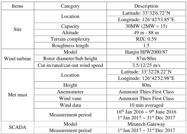
The porous flat circular disc is placed perpendicular to the air flow and acts as a momentum sink. The mass of flow does not change when passing though the actuator disc, but the flow velocity will decrease. The air flow acts as an incompressible fluid and expands to a cylinder with a larger diameter than the disc, which is described in Fig. 2 with streamlines of air flow.

(21)

10

Fig. 2 Streamlines of air flow passes though the actuator disc [20]

The streamlines pass through the disc and the wind speed deficit appears. That is, the wind speed V at the rotor is lower than the wind speed V1 before reaching the

turbine rotor. The theory explains this operation by axial induction factor, a, with the following equation:

𝑉 = (1 − 𝑎)𝑉1 (1)

The thrust coefficient CT for the rotor disc is defined by the following equation:

𝐶𝑇 = 𝑇 1 2𝜌𝑉1

2_𝐴 (2)

Where, T is thrust force, 𝜌 is air density. V1 is free stream velocity and A is

(22)

11 3.3 Turbulence intensity

The flow passes through the wind turbine rotor, which leads the turbulence level behind the rotor to increase, while the wind speed reduces. Turbulence intensity is defined by ratio of standard deviation of the wind speed to mean wind speed. In ANSYS CFX, turbulence intensity, TI, is calculated by the following equation [10]:

TI =√

2 3𝐾

𝑉 (3)

Where, K is turbulence kinetic energy, V is local wind speed.

The Shear Stress Transport (SST) model is the combination of the k-ε model and the k-ω model to accomplish the formulation of an optimal model for a wide range of applications. In addition, the SST model presents the adjustment of the eddy viscosity definition [22]. The SST turbulence model is the default option for the WindModeller simulations.

(23)

12 3.4 Atmospheric stability

Atmosphere is the three-dimensional fluid that contains the air. As the air moves through the atmosphere, the climate change will be created by air movements [23]. Stability is highly related to the air temperature with height. The temperature change with height is called the dry adiabatic lapse rate, Г_𝑑, which is expressed in the following equation:

Г_𝑑 =−𝑑𝑇

𝑑𝑧 ≡ 𝑐𝑝

𝑔 = 9.8℃/𝑘𝑚 (4)

Where, T is temperature, z is height, cp is specific heat at constant pressure and

g is gravitational constant. As seen in the equation, the air temperature will decrease approximately 10℃ at 1km elevation, which means the temperature will drop 1℃ every 100m [24].

The pressure and temperature can be combined into one variable which is the potential temperature, Ɵ. Ɵ = T (𝑝0 𝑝) 𝑅 𝑐𝑝 (5) Where, T is the temperature at a given height, p0 is the pressure at the surface,

p is the pressure at the same height as the temperature, T, and R is the gas constant. There are 3 states the atmosphere can be in which is neutral stable and unstable. During the neutral condition, the potential temperature is constant with the height. The atmosphere is in stable condition if the ratio of the potential temperature to the height is positive. On the other hand, an unstable condition has a negative ratio of the potential temperature to the height.

(24)

13

Neutral atmosphere has the same lapse rate as the surroundings. If the air has lifted through the neutral layer, the air parcel temperature and pressure is exactly the same as the temperature and pressure of the surroundings at every air height. Therefore, the air mass is not buoyant.

Stable atmosphere is more likely to stay without change. The air parcel of the stable condition easily goes back to the original position after climate changes. Also, if the air mass is lifted, it has negative buoyancy which means the air wants to sink back to its original position. On the other hand, if the air is pressed down, it has positive buoyancy which means the air wants to rise back.

Unstable atmosphere has the tendency to fluctuate. When the air mass has lifted, it is likely to continue going upward even if the pushing force is gone. The air mass has less lapse rate than the environment lapse rate [23].

(25)

14

4. Results and discussion

The conditions for the WindModeller Simulation for this study are presented in Table 3. The terrain with 2,000 to 5,000m of radius and 500 to 1,000m of height was created, and horizontal and vertical grid resolutions were 40m and 30m, respectively. To obtain a more accurate calculation result for the atmospheric boundary layer, the first vertical cell was started at 7m above the ground, and the following at 30m and the vertical cells from the next increased with a 1.15 expansion factor.

The inflow boundary conditions V0 are given in the following equation [25]:

𝑉₀ = 𝑉

𝑘Ln ( 𝑧

𝑧0) (6)

Where, V is the velocity at the reference height, and k is the Von Karman constant. And z0 is the roughness length.

The turbulence intensity over the terrain is calculated using Eq (3).

4.1 Wake influence between wind turbines

Since the prevailing wind direction on DBK wind farm is from the northwest, the wind direction of 314 degrees was input for the simulation. The wind speed of 9.3m/s at 80m a.g.l. was used as a reference wind speed. The actuator disc model was used to predict the wake behind wind turbines. The turbulence model of SST was used with the 𝐶_𝜇Constant of 0.03 and turbulence decay rate of 0.6.

(26)

15

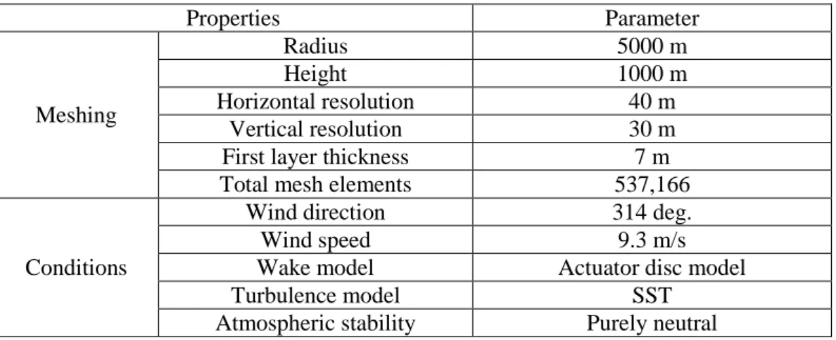
Table 3 Parameters used in WindModeller for wake simulation

Properties Parameter Meshing Radius 5000 m Height 1000 m Horizontal resolution 40 m Vertical resolution 30 m

First layer thickness 7 m

Total mesh elements 537,166

Conditions

Wind direction 314 deg.

Wind speed 9.3 m/s

Wake model Actuator disc model

Turbulence model SST

Atmospheric stability Purely neutral

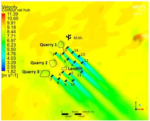
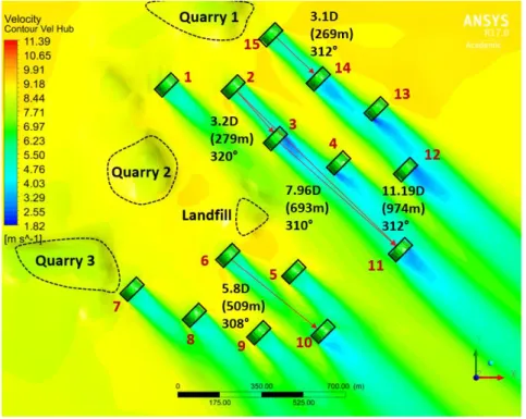
Fig. 3 shows the velocity distribution at the hub height of 80m. The locations of the wind turbines are expressed by black rectangles with the turbine numbers, and the met mast (M.M) is also illustrated as well. The lower wind speeds are observed over the quarries around the wind farm.

It is clear that the upstream turbines are not affected by the wake. The downstream turbines are affected by the wake from the upstream turbines. The wakes from turbines no. 2 and 15 give direct impact on turbines no. 3 and 14. Turbines no. 11 and 12 are influenced by the wake from the multiple upstream turbines. The wakes behind turbines no. 3 and 14 have a half effect on turbines no. 4 and 13, respectively. The wake effect behind the turbines goes downstream several kilometers. The velocity immediately behind turbines no. 3 and 14 decreases up to 40% of those at the upstream wind turbines.

(27)

16

Fig. 3 Velocity distribution at hub height under wind direction of 314deg.

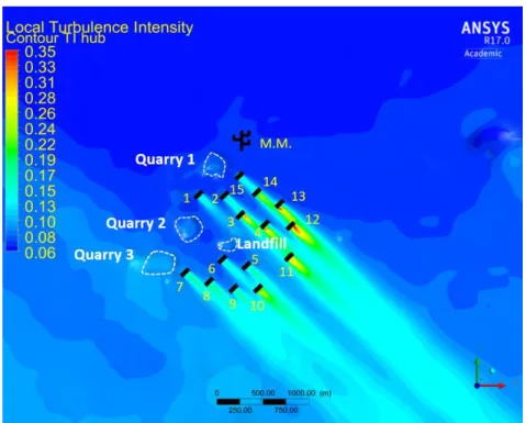
Fig. 4 shows the turbulence intensity distribution at a hub height of 80m a.g.l. A slightly higher turbulence intensity appears over the quarries in the wind farm. Strong turbulence intensity can be found in the wake behind multiple wind turbines. The effect of the turbulence intensity persists for several kilometers downstream following the same trend as the velocity. Turbines no. 12 and 13 have a high turbulence intensity on one side of the rotor. Immediately behind the turbine rotor, the turbulence intensity increases, while velocity decreases as shown in Fig. 3. The turbulence intensity increases up to 0.42 immediately behind turbine no. 13. Also, the turbines experiencing the wake from multiple turbines show a very high turbulence intensity compared to other turbines.

(28)

17

Fig. 4 Turbulence intensity distribution at hub height under a wind direction of 314 degrees

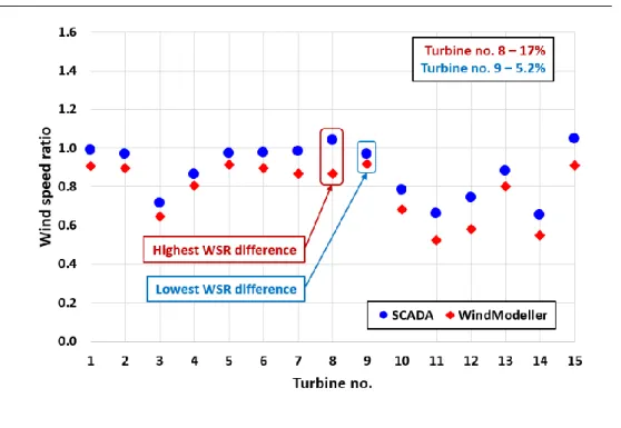
The predicted wind speed was extracted from the wind speed data immediately in front of the actuator disc from the results of the WindModeller simulation, while the actual wind speed was collected from the SCADA system of the wind farm. Fig. 5 shows the comparison of actual and simulated wind speed ratios for both the simulated and the actual wind farm. The velocity ratio is the ratio of the nacelle wind speed to mast wind speed which is given by the following equation:

Velocity Ratio =𝑁𝑎𝑐𝑒𝑙𝑙𝑒 𝑊𝑖𝑛𝑑 𝑆𝑝𝑒𝑒𝑑

𝑀𝑎𝑠𝑡 𝑊𝑖𝑛𝑑 𝑆𝑝𝑒𝑒𝑑 (7)

Overall, the wake predicted by the WindModeller is higher than the actual wake from the SCADA system. A 10% difference on average was found between the actual and the simulated wind speed ratios. There are a few reasons for the difference

(29)

18

between simulation and measured data. The main reason is because the porous disc converts the flow into turbulence immediately downstream, while the rotating rotor derives the flow into energy downstream. The biggest difference between them appeared on turbine no. 8, which was about 17%, while turbine no. 9 had the smallest difference of 5.2%.

The turbines, affected by the wake behind multiple turbines, have lower wind speed ratios compared with the other turbines. Since turbine no. 11 was affected by the wake from turbines no. 2 and 3, the simulated and the actual wind speed ratios were very low, which were less than 70%. On the other hand, turbine no. 14 also had significantly low ratios because it was directly influenced by the wake from turbine no. 15. Since the distance between the two turbines is comparatively short, which is only 3.1 times the rotor diameter, the speed ratios greatly decreased. However, the front row of turbines showed wind speed ratios of around 1.0, because they were not affected by the wake.

(30)

19

Fig. 5 Comparison of actual and simulated wind speed ratios of each turbine

Fig. 6 shows the distance between the upstream and downstream turbines, which stems from an enlargement of Fig. 2. The figure shows that the wake effect changes depending on the distance between the turbines. In order to clarify the wake effect with the distance between the turbines, the representative wakes behind the single and multiple turbines were chosen on the wind farm. Single wakes were generated behind turbines no. 6 and 15, which had an influence on turbines no. 10 and 14, respectively. The distances between each pair of turbines are 5.8 D and 3.1 D, respectively. The wake was created by turbine no. 3 which was affected by the single wake from turbine no. 2, which had an influence on turbine no. 11. The distance between turbines no. 2 and 11 is 11.19D, and each distance between the turbines is shown in the Figure.

(31)

20

Fig. 6 Velocity distribution at hub height under a wind direction of 314 degrees and the distance between the turbines

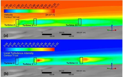
A vertical cut was made along the line at 312 degrees shown in Fig. 6 for clarifying the wake effect from turbines no. 2, 3 and 11. Fig. 7 presents the vertical velocity and turbulence intensity distributions. The velocity decreased behind turbine no. 2, and further decreased behind turbine no. 3. However, the velocity increased more and more by mixing with the surrounding air within the distance between turbines no. 3 and 11. The velocity further decreased behind turbine no. 11, which then increased by mixing with the surrounding air.

The vertical turbulence intensity distribution was opposite to the vertical velocity distribution. The turbulence intensity immediately behind the turbine rotor was higher than the others. As the distance increased, the turbulence intensity

(32)

21

decreased due to an increase of velocity with the further distance from the turbine rotor as shown in Fig. 7.

Fig. 7 Velocity and turbulence intensity distribution on a 312 degree vertical plane

Fig. 8 shows the comparison of the actual and the simulated wind speed ratios for a single wake with the distance between turbines. The actual wind speed ratio was about 10% higher than the simulated wind speed ratio. The actual and the simulated velocities increased as the distance between the turbines increased. For the distance of 3.1 D and 5.8 D, the actual wind speed ratios decreased by 35% and 22%, respectively.

(a)

(33)

22

Fig. 8 Comparison of actual and simulated wind speed ratios for a single wake with the distance between turbines

Fig. 9 shows the comparison of the actual and the simulated wind speed ratios for the various wakes from turbines. As shown in Fig. 6, since turbine no. 2 is located in the front row facing the wind, turbine no. 3 is affected by the single wake from turbine no. 2. Turbine no. 11 is also impacted by turbines no. 2 and 3. The simulated wind speed ratio was about 11% lower than the actual wind speed ratio. The wind speed ratio of turbine no. 11 was lower than the others. The actual wind speed ratios decreased by 28% and 34% for turbines no. 3 and 11, respectively.

(34)

23

Fig. 9 Comparison of actual and simulated wind speed ratios for the various wakes from turbines

4.2 Wake influence from nearby obstacles

There are two hills and three quarries in and around the wind farm. First of all, the 2 cases for each hill was simulated and the results were compared with the SCADA data of the wind farm to investigate the wake effect from the hills and quarries. This part of the study did not include simulation for the landfill. Due to the surrounding quarries and turbines, it was impossible to analyse the only landfill.

The wind speed of 9.1m/s at 80m a.g.l was used as the reference wind speed. As mentioned in the previous chapter, the actuator disc and SST turbulence models were used to predict the wake effect and the turbulence intensity, respectively. Table

(35)

24

4 shows the parameter for simulation of the case for hill 1.

Table 4 Parameters used in WindModeller for simulation for hill 1

Conditions

Wind speed 9.1 m/s

Fig. 10 shows turbine layout and nearby obstacles with altitude. Hill 1 and the quarries are marked with dashes. Hill 1 is about 2.5km away from turbine no. 1.

(36)

25 Fig. 11 Velocity distribution at hub height

Fig. 11 shows the velocity distribution at hub height. Turbine no. 1 and 15 are under the direct influence of hill 1. On the other hand, turbines no. 6 and 7 are not receiving any wake from the hill which shows possibility of comparing the wake influence from hill 1. In order to clarify the wake from the hill, 2 sets of cuts were extracted from the simulation results, which included the hill and turbines no. 1 and 6 with direction of 288 degrees.

Fig. 12 shows the 2 vertical plane cuts with turbine no 1, hill 1 and turbine no. 6. The first cut shows the direct wake from hill 1 and second cut shows the wake free flow to turbine no. 1. Fig. 12a presents the velocity decrease behind hill 1, while Fig. 12b shows the constant velocity distribution.

(37)

26

Fig. 13 shows the comparison of wind speed ratios at the turbine under wake effect and the turbine under free wake flow. The ratio predicted by the WindModeller was similar to that from the SCADA data. In the case of turbine no. 1, the wake effect occurred from hill 1. The predicted ratios were 0.9 and 0.81 for the WindModeller and SCADA, respectively. As for turbine no. 6 without the hill wake effect, the predicted ratio was in near proximity with the actual ratio, which were 1 and 0.95 for the WindModeller and SCADA, respectively. This means that hill 1 caused a wake effect loss of 10% in reality and a wake effect loss of 14% in the WindModeller which effectively caught the wake effect of hill 1.

(a)

(38)

27

Fig. 13 Comparison of actual and simulated wind speed ratios for turbine under wake effect from hill 1 and turbine under free flow

Next, the simulation of the hill 2 wake effect was conducted with a wind speed of 9.4m/s at 80 a.g.l and used as the reference speed. Table 5 shows the parameters for simulation of the case for hill 2.

Table 5 Parameters used in WindModeller for simulation for hill 2

Conditions

Wind speed 9.4 m/s

(39)

28

Fig. 14 shows the wind farm layout and nearby obstacles with the altitude. On this layout of the wind farm, hill 2 and the quarries are marked with black dashes. The distance between hill 2 and the wind farm is about 2.1 km.

Fig. 15 shows the velocity distribution at hub height. In this case, turbine no. 15 is under wake free flow and turbine no. 12 is under the direct wake influence of hill 2. In order to clarify the wake from the hill, 2 sets of cuts were extracted from the simulation results, which included the hill and turbines no. 12 and 15 with a direction of 66 degrees.

Fig. 16 shows the 2 vertical plane cuts for turbine no. 12 which is under direct wake effect and turbine no. 15 which is under wake free flow. Fig. 16a presents the velocity decrease behind hill 1, while Fig. 16b shows the constant velocity distribution.

(40)

29 Fig. 15 Velocity distribution at hub height

Fig. 16 Velocity distribution of 2 cuts on a 66 degree vertical plane (a)

(41)

30

Fig. 17 shows the comparison of wind speed ratios for the turbines under wake influence and under wake free flow. The ratio predicted by the WindModeller was similar to that from the SCADA data. In the case of turbine no. 12, wake effect occurred from hill 2. The predicted ratios were 0.91 and 0.9 for the WindModeller and SCADA, respectively. As for turbine no. 15 without the hill wake effect, the predicted ratios were 0.99 and 1 for the WindModeller and SCADA, respectively. This means that hill 2 caused a wake effect loss of 8% in reality and the WindModeller caught the wake effect of hill 2. And the predicted ratios for the WindModeller and SCADA were in near proximity with a 1% difference.

Fig.17 Comparison of actual and simulated wind speed ratios for turbine under wake effect from hill 2 and turbine under free flow

(42)

31

Next, a simulation of influence from the quarry was done with a wind speed of 9.3m/s at 80 a.g.l and used as the reference speed. Fig. 18 shows the wind farm layout and location of quarries including altitude. In the figure, the quarry is quite visible and marked with black dashes. Quarry 1 is relatively deeper and larger than the other 2 quarries. Table 6 shows the parameters for simulation of the case for quarry 1.

Table 6 Parameters used in WindModeller for simulation for quarry 1

Conditions

Wind speed 9.3 m/s

Fig. 19 shows the velocity distribution of the overall wind farm. The quarries are identified, where the lower wind speed is found. The vertical cut was made with turbine no. 15 located immediately behind the biggest quarry and the turbine under free flow to identify the velocity change through the quarry and compare the differences of flow with and without wake influence.

(43)

32

Fig. 18 Turbine layout and location of quarries including altitude

(44)

33

Fig. 20 shows the velocity distribution of vertical cuts on turbines no. 15 and 6. The first cut shows direct influence from quarry 1 and the second cut shows free flow to turbine no. 6. Fig. 20a presents the velocity decrease over the quarry, while Fig. 20b shows the constant velocity distribution.

Fig. 21 shows the wind speed ratios between turbine no. 6 without a quarry and turbine no. 15 with quarry 1. The ratio predicted by the WindModeller was similar to that from the SCADA data. In the case with no quarry, the two ratios were close to 1, which means no wind speed deficit occurred from the surroundings. For turbine no. 15 with quarry 1, the predicted ratio was in close proximity with the actual ratio, which were 0.96 and 0.92 for the WindModeller and SCADA, respectively. As for turbine no. 6 without a quarry, the predicted ratio was also in close proximity with the actual ratio, which were 1.07 and 0.95 for the WindModeller and SCADA, respectively. This concludes that quarry 1 caused the wind speed deficit of 3% in reality and the wind speed deficit of 11% in the WindModeller.

(45)

34

Fig. 21 Comparison of actual and simulated wind speed ratios for turbine under flow with wind speed deficit and turbine under free flow

(a)

(46)

35 4.3 Atmospheric stability

On the wind farm site, the temperature conditions for atmospheric stability analysis were not measured. To understand the difference between stable and unstable atmospheric conditions, the met mast data was binned by day and night. The shear exponent and the turbulence intensity were analysed using the met mast data. The results are presented in Fig. 22. The increased shear exponent and the reduced turbulence intensity were found during night time, while the opposite trend was obtained at day time. These trends imply surface atmospheric stability affects the wind flow at a site.

Since the mast was placed near the wind turbines, the mast had a disturbed sector by the wake behind the turbines from 104.1 to 246.6 degrees. The measured mast wind speed data, from 7.5m/s to 17.5m/s of wind speeds, was chosen for this study. In the disturbed sector, the higher shear exponent and turbulence intensity were analysed for this study. The reason for the high shear exponent and turbulence intensity in the disturbed sector, should consider both the atmosphere stability and wake effect from the wind turbines.

A CFD simulation of atmospheric stability was done with the WindModeller. In this part of the study, met mast data was used for 6 months (Jan 16th_{~ Jun 9}th_{, 2016).}

Atmospheric stability was modelled with the transport equation for potential temperature, considering the ISO standard potential temperature gradient above the boundary layer, and surface stability was modelled with potential temperature offset at the ground. The other parameters used for simulation are listed in Table 7. The wind

(47)

36

speed of 7.5m/s to 17.5m/s at 80m a.g.l were used as the reference wind speed. In addition, the wind direction was analysed at every 10 degrees. Compared to previous simulations, the reference speed and wind directions were examined over wider ranges for this simulation.

(48)

37

Table 7 Parameters used in WindModeller for analysis of atmospheric stability

Conditions

Wind direction 0~360 degrees with 10 degrees bin Wind speed 7.5m/s, 10m/s, 12.5m/s, 15m/s, 17.5m/s

Atmospheric stability Purely neutral, Neutral, Stable, Unstable

The purely neutral condition is the condition that does not consider any atmospheric stability at the terrain. This means there is no temperature change with the height above the ground. This type of condition does not really exist in a real atmospheric condition.

The simulation with neutral condition was carried out under the potential temperature gradient, considering the ISO standard potential temperature (3.3e-3K/m) as the default. The simulation for stable condition was conducted under positive potential temperature gradient above boundary layer with positive in the surface layer which is considered as the negative temperature offset. The simulation for unstable condition is performed under the potential temperature gradient with negative gradient above the boundary layer with negative surface layer which is considered as the positive temperature offset [27].

(49)

38

Fig. 23 shows three temperature measurement points for atmospheric stability analysis. Points 1 and 2 are located at the entrance of wind flow, and at the middle of the terrain radius which is 2.5km away from the entrance, respectively. Point 3 is positioned at 300m behind turbine no. 10. Temperature and wind shear were analysed at these 3 points.

(50)

39

Fig.24 shows the temperature with height a.g.l under various atmospheric conditions at Points 1 and 2. The temperature offsets were input, which were ±2K from 288K for stable to unstable conditions. The left figure shows the temperature under various stability conditions at the entrance. The temperature change with height appears the same as the input condition. The right figure shows the temperature change with the height at 2.5km away from the entrance. As the flow distance got further, the input temperature was mixed with the surrounding temperature, which led to a smoother temperature gradation.

Fig. 24 Temperature change with height under various atmospheric conditions at Point 1 and Point 2

(51)

40

Fig. 25 shows the wind shear with height at various atmospheric stability conditions. No wake effect was presented at points 1 and 2 at all of the atmospheric stability conditions. Wind speeds at points 1 and 2 have very slight differences for every atmospheric stability condition. Wind shear gradient is the highest at purely neutral condition among all the conditions. The wind shear gradient at neutral condition is higher than the unstable condition and lower than the stable condition.

Unlike points 1 and 2, point 3 was under wake effect from turbine no. 10 which was presented differently depending on atmospheric stability conditions. The wind speed at hub height for the purely neutral condition is higher than the purely neutral condition. Since the purely neutral condition does not consider atmospheric stability, the wind speed at hub height for other atmospheric stability conditions except the stable condition is higher than the purely neutral condition. Also, the wind speed at hub height is lowest at the unstable condition and highest at the stable condition. The wind speed at hub height at the neutral condition is lower than the unstable condition and higher than the stable condition. Overall, the wind profile was different depending on the atmospheric stability conditions.

(52)

41

Fig. 25 Wind shear at various atmospheric stability conditions

For 360 degrees with 10-degree bins, the sensitivity of the simulated shear exponent and turbulence intensity to atmospheric stability is presented in Fig. 26. ±2K for the surface temperature offset was given to present unstable and stable conditions. At the different atmospheric conditions, simulation results of the shear exponent are at positive correlation to the real exponent from the mast data in the undisturbed sector. However, the simulation results of turbulence intensity do not correlate with that from the measured data. The results were underestimated in most of the undisturbed sectors, while a few of the simulation results were highly underestimated at the disturbed sector.

(53)

42

Fig. 26 Shear exponent and turbulence intensity data from Mast compared with simulation result (simulation carried out with reference speed of 10m/s)

(54)

43

In Figs. 27 and 28, various wind speeds were analysed and compared with measurement data. Fig. 27 shows shear exponent data from the mast compared with predicted shear exponent with a wide range of wind speeds at various conditions. Since the purely neutral condition does not exist in real atmospheric condition, simulation results present insignificant difference depending on wind speeds in the undisturbed sector. As for the unstable condition, the shear exponent shows an opposite trend to wind speed and all the simulation results are predicted inside one standard deviation of the measured data. On the other hand, predicted the shear exponent for the stable condition is higher than the average measured shear exponent at the wind direction from 260 to 360 degrees. Eventually, the predicted shear exponent for most of the neutral conditions are well matched with measured data.

Fig. 28 presents turbulence intensity from the mast compared with simulation results with a wide range of wind speeds at various conditions. Overall the predicted turbulence intensity was underestimated at all the atmospheric conditions. As mentioned above, the predicted turbulence intensity was the same at different wind speeds at the purely neutral condition. In the unstable condition, 17.5m/s of reference wind speed presented the lowest turbulence intensity, while, 7.5m/s of reference wind speed showed the highest turbulence intensity. Nevertheless, the predicted turbulence intensity was lowest for the stable condition compared to the predicted turbulence intensity for unstable and neutral conditions. However, simulation results of the neutral condition were at halfway between the stable and unstable conditions.

(55)

44 Fig. 27 Sh ea r expo nen t da ta f rom m as t com pa red t o s im ul at ion res u lt s wi th r ang e of r ef er en ce w in d spe eds at v ar iab le c o ndi ti ons

(56)

45 Fig. 28 T u rbu len ce i nt ensi ty dat a f rom m as t com par ed t o s im ul at ion r es u lt s wit h r ang e of r ef er en ce w in d spe eds a t v ar iabl e c ond it ion s

(57)

46

5. Conclusions

Through CFD analysis using the WindModeller, the wake effects from neighbouring wind turbines and nearby hills were evaluated in DBK wind farm, and the predicted wake effect was compared to the actual wind speeds measured from the met mast and SCADA system. Wind speed deficit caused by quarry 1 in the farm was estimated by the WindModeller, which was comparatively evaluated with real wind speeds. Additionally, the wind flow sensitivity was analysed under various atmospheric stability conditions. The results are as follows:

1) It was found that the wind speed ratio predicted by the WindModeller was about 10% lower than the real wind speed ratio from the SCADA data under the wind farm site conditions.

2) The actual and the simulated wind speed ratios decreased by 35% and 45%, respectively, for the distance of 3.1 D, while they reduced by 22% and 32%, respectively, for the distance of 5.8 D.

3) Turbine no. 11 showed a 34% loss for the actual wind speed ratio and a 48% loss for the simulated wind speed ratio because of the wake from upstream turbines no. 2 and 3.

4) It was confirmed that the neighbouring hills 1 and 2, and quarry 1 caused wind speed deficits in the wind farm. The wind speed deficits of 10% and 8% were predicted due to the wakes behind hills 1 and 2 by the WindModeller, which were in close proximity with real wind speed deficits of 14% and 9%,

(58)

47

respectively. Quarry 1 resulted in a wind speed deficit of 3% from the SCADA data analysis, while a wind speed deficit of 11% was found from the WindModeller simulation.

5) It was clear that atmospheric stability had a significant effect on the wind shear and the turbulence intensity in the wind farm. That is, actual wind data analysis showed that the wind shear exponent factor during night time was higher than that during day time, while the opposite trend was found for the turbulence intensity. This tendency based on actual wind data analysis was the same as that from the WindModeller analysis.

(59)

48

References

[1] E. S. Politis, J. Prospathopoulos, D. Cabezon, K. S. Hansen, P. K. Chaviaropoulos, R. J. Barthelmie, Modelling wake effects in large wind farms in complex terrain: the problem, the methods, and the issues, Wind Energy 15, pp. 161-182, 2015 [2] P. Mckay, R. Carriveau, D. S-K. Ting, T. Newson, Turbine wake dynamics,

Advances in wind power, Chapter 3, 2012

[3] J. Bartl, F. Pierella, L. Sæ tran, Wake measurements behind an array of two model wind turbines, Energy Procedia 24, pp.305 – 312, 2012

[4] C. Montavon, C. Rodaway, P. Housley, I. Jones, Sensitivity of wind flow to atmospheric stability for a complex site with multiple masts, EWEA, 2014 [5] A. Pena, P. E. Rethore, O. Rathmann, Modeling large offshore wind farms under

different atmospheric stability regimes with the Park wake model, Renewable Energy 70, pp. 164-171

[6] WAsP user manual, 2005

[7] Ko Kyung-Nam, Huh Jong-Chul, Estimation of the wake caused by wind turbine and complex terrain by CFD wind farm modelling, Journal of the Korean Solar Energy Society 31, pp.19-26, 2011

[8] R. Mikkelsen, Actuator Disc Methods Applied to Wind Turbines, 2003

[9] P. Argyle, S. Watson, C. Montavon, I. Jones, M. Smith, Turbulence intensity within large offshore wind farms, EWEC Processing, 2015

(60)

49

[10] C. Montavon, G. Ryan, C. Allen, P. Housley, C. Staples and I. Jones, Comparison of meshing approaches and RANS turbulence models performance for flows over complex terrain, EWEC Processing, 2010

[11] ANSYS CFX – Solver Theory Guide, pp.102-103, 2011

[12] P. Argyle, Computational fluid dynamics modelling of wind turbine wake losses in large offshore wind farms, incorporating atmospheric stability, 2014 [13] S. Roma Solanellas, C. Montavon, D. Madueno, A. Moragrega, S. Espana,

Sensitivity of wake losses to wind turbine diameter for a offshore wind farm, EWEC Processing, 2014

[14] C. Montavon, I. Jones, C. Sander, Accounting for stability effects in the simulation of large array losses, EWEC Processing, 2012

[15] C. Montavon, I. Jones, D. Malins, C. Strachan, R. Spence, Modelling of wind speed and turbulence intensity for a forested site in complex terrain, EWEC Processing, 2012

[16] WindModeller user manual, ANSYS, 2014

[17] D. Sturge, D. Sobotta, R. Howell, A. While, J. Lou, A hybrid actuator disc – Full rotor CFD methodology for modelling the effects of wind turbine wake interactions on performance, Renewable energy 8-, pp.525-537, 2015

[18] V. M. M. G. Gosta Gomes, J. M. L. M. Palma, A. Silva Lopes, Improving actuator disc wake model, The science of making torque from wind (TORQUE), 2014

[19] G. Crasto, A. R. Gravdahl, F. Castellani, E. Piccioni, Wake modelling with the actuator disc concept, Energy procedia 24, pp.385-392, 2012

(61)

50

[20] Bhaskara, For explanation of Betz’s law, 2015

[21] Martin O. L. Hansen, Aerodynamics of wind turbines, 2015

[22] F, Menter, J. Carregal Ferriera, T. Esch, B. Konno, The SST turbulence model with improved wall treatments for heat transfer predictions in gas turbines, Processing of the International gas turbine congress, 2003

[23] O. M. Almethen, Z. S. Aldaithan, The state of atmosphere stability and instability effects on air quality, IJES 6 (2017), pp.2319-1805

[24] L. Landberg, Meteorology for Wind Energy: An Introduction, 2015, Chapter 4 [25] C. Montavon, I. Jones, C. Staples, C. Strachan, I. Gutierrez, Practical issues in

the use of CFD for modelling wind farms, EWEC Processing, 2009 [26] C. Montavon, Atmospheric stability, ANSYS

[27] S. Wharton, J. K. Lundquist, Atmospheric stability affects wind turbine power collection, Environmental research letters, 2012

(62)

51

감사의 글

큰 결심을 하고 몽골을 떠난 지 벌써 2년이란 시간이 흘렀습니다. 많은 것을 경험하고 배울 수 있었던 뜻깊은 시간이었습니다. 힘든 시간도 많았고 답답할 때 도 있었지만 풍력공학부 식구들이 있었기에, 마지막까지 의지하고 버틸 수 있었 고 마침내 석사학위 논문을 완성할 수 있었습니다. 그동안 도움을 주신 많은 분들 께 이 자리를 빌려 감사의 인사를 전하고자 합니다. 논문이 무엇인지 가르쳐주시고 항상 부족한 저를 믿어주시며 연구지도를 통 하여 바른 방향으로 나아갈 수 있도록 도와주시는 지도교수 고경남 교수님, 제주 대학교 대학원 풍력공학부 설립 후 발전할 수 있도록 불철주야 노력하시고 많은 학생들이 최적의 교육환경에서 공부할 수 있도록 헌신해 주시는 허종철 교수님, 수준 높은 자료와 열정적인 강의를 통하여 풍력에 대한 많은 지식을 알려주신 김 범석 교수님 모두 감사드립니다. 타지인 한국에서의 생활을 적응할 수 있도록 도와주신 풍력단지설계 연구 실 오빠들, 동헌이 오빠, 동범이 오빠, 진혁이 오빠, 건우 오빠, 진석이 오빠, 바쁜 와중에도 찾아가면 항상 군말 없이 도와주셔서 감사드립니다. 그리고 첫날부터 한 국의 문화와 생활을 가르쳐주신 병택이 오빠 모두 감사드립니다. 제주도에 와서 만나게 된 나의 고향 친구동생들, 홀란, 사라, 그리고 공이, 모두 항상 함께 있어주고 힘을 낼 수 있도록 도와주어 감사드립니다.

(63)

52 마지막으로 평생 나를 항상 믿고 응원해주는 우리가족, 아버지, 어머니, 오 빠, 동생, 그리고 몽골에서 응원하고 있는 든든한 나의 친구들, Baaska와 Ayush 모두 진심으로 감사하고 보고 싶습니다. 그리고 사랑합니다. 2018년 12월 01일 투멘바야르 운다르마 올림

(64)