Development of In-Situ Monitoring System for measuring soil gas

(1)

Development of In-Situ Monitoring System for measuring soil gas

토양가스 측정을 위한 현장 모니터링 시스템 개발

Yu, Chan* ․ Lee, Jong-Beom 유 찬 경상대( ) ․ 이종범 도건이엔씨( ) Abstract 생물학적 통풍법은 유류오염 지역에 자주 적용되는 정화공법이다 이 과정은 지중에 산소를 충. 분히 공급함으로서 토착 미생물에 의한 오염성분의 분해를 가능하게 한다 따라서 이 공법의 적용. 시 공정진행에 따른 공법의 효율성 분석과 장기적인 정화효율 예측을 위한 지중 가스성분의 모니 터링 시스템 도입이 매우 중요하다 그러나 우리나라에서는 아직 그 적용사례가 보고된 바 없다. . 따라서 본 연구에서는 현장에서 토양가스 성분의 변화를 모니터링할 수 있는 시스템을 개발하여 적용한 사례를 시스템의 구성과 측정방법 관측결과를 중심으로 소개하였다 현장적용 결과는 토, . 양가스 모니터링 시스템은 운용 시작 후 6개월동안 센서나 측정장비에서 문제가 발생되지 않았으 며 공정관리를 위한 공법효율성 분석에 필요한 자료를 지속적으로 제공하고 있다, . I. Introduction

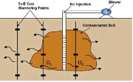
Bioventing is a proven technology that stimulates the natural in situ biodegradation of petroleum hydrocarbons in soil by providing oxygen to native soil microorganisms. In contrast to soil vapor extraction(SVE), bioventing utilizes low air-injection flow rates to provide only enough oxygen to sustain microbial activity. Oxygen is most commonly supplied through direct air injection into contaminated vadose-zone soils via vertical or horizontal vent wells. Oxygen serves as a primary electron acceptor for soil microorganisms employed in the degradation of both refined and natural hydrocarbons. Following a hydrocarbon spill, soil microorganisms begin to use available soil gas oxygen. As the population of fuel-degrading microorganisms increases, the supply of soil gas oxygen is often depleted, creating an anaerobic volume of contaminated soil. Under anaerobic conditions, fuel biodegradation generally proceeds at significantly slower rates. In some cases, aerobic biodegradation will continue because the diffusion or advection of oxygen into soils from the atmosphere exceeds biological oxygen utilization rates. Under these circumstances the site is naturally aerated, and the hydrocarbons will be naturally attenuated over time. In addition to biodegradation of adsorbed fuel residuals, volatile organic compounds(VOCs) also are biodegraded as vapors move slowly through biologically active soils.

Generally, monitoring is performed during the operational phase to evaluate whether the remediation equipment is functioning as designed and whether the remediation is progressing as predicted. In this case, the use of soil gas to determine bioventing performance and bioventing progress has several economic and technical advantages over more traditional drilling and soil sampling techniques. Thus the proper soil gas, not just off-gas, monitoring system must be developed and located strategically inside and outside of the contaminated soil volume to ensure the adequate aeration in subsurface contaminated zone(see Fig. 1).

In this study in-situ soil gas monitoring system was developed and presented the results of application in the field that was performing the remediation project by bioventing method.

(2)

Fig. 1 Typcal bioventing system

II. Development of soil gas monitoring system

The chemical composition of soil gas can vary considerably from atmospheric composition as a result of biological and mineral reactions in the soil. Although numerous compounds and elements may be present in soil gas as a result of specific soil and bedrock geochemistry, three indicators are of particular interest in the bioventing context: oxygen, carbon dioxide, and. hydrocarbon vapors. The soil gas concentrations of these indicators in relation to atmospheric air and uncontaminated background soils can provide valuable information on the ongoing natural biodegradation of hydrocarbon contaminants and the potential for bioventing to enhance the rate of natural biodegradation.

There are many possible procedures for monitoring the progress of bioventing. These processes include point source monitoring, use of helium tracers, finger printing and continuous monitoring using sensor technology (Hinchee, Douglas and Ong, 1995). It is our opinion that the use of subsurface oxygen, carbon dioxide and temperature sensors in addition to soil sampling is the most appropriate monitoring scheme to track the progress of the remediation of the soil. A monitoring process using various sensors offers the possibility of continuous, uninterrupted monitoring of the average respiration rate and the activity of microbiota metabolic in the air flow path.

The sensor consists of an electrochemical cell which monitors the oxygen, carbon dioxide content of the media continuously (Hinchee, Douglas and Ong, 1995). Sensors were installed at various depths, between the surface of the soil and the 6 or 7m points. We were installed more sensors in the spots than in the surrounding contaminated areas. The sensors were packed with sand and isolated. This method of installation was chosen over simply hanging the sensors in existing wells because it generally provides more accurate results(Hinchee, Douglas and Ong, 1995). It is necessary to take an initial reading of oxygen levels as soon as the installation is complete. In addition, a control sample from a nearby unaffected area should be taken to establish the normal chemistry of the soil(North West Soil Research, 1979). The soil gas monitoring system was installed as Fig. 2 and photo 1 and the specification of analyzers and sensor which was used to compose the soil gas monitoring system was as Table

(3)

1. 1 ,0 0 0 1 ,0 0 0 1 ,0 0 0 1 ,0 0 0 … … . 5 ,0 0 0 ~ 6 ,0 0 0 m m Casagrande Tips Protect Cover Thermometer P.V.C Pipe 1, 2, 3, 4, 5, ….m 1 ,0 0 0 1 ,0 0 0 1 ,0 0 0 1 ,0 0 0 … … . 5 ,0 0 0 ~ 6 ,0 0 0 m m Casagrande Tips Protect Cover Thermometer P.V.C Pipe 1, 2, 3, 4, 5, ….m

Fig. 2 Diagrammatic representation of soil gas monitoring system

(a) assemblage (b) drilling

(4)

Photo. 1 Installation processes of sensors Table 1. Specification of equipments & sensor

Item Specification Remarks

Oxygen meter Gases detected : OxygenDetection Principle : Galvanic cell Range : 0-40% VOL Alarm at below 18% IAQ monitor CO2 : 0 to 5000ppm Temperature : 32 to 140°F Relative Humidity : 5 to 95% RH % Outside Air : 0 to 100% CO : 0~500ppm Thermo meter (KM320)

Sensor Type : Thermocouple Type K Measurement Range : -50℃ ~ +1300℃

Resolution : 1℃

Connector Type : Sub-miniature

Operating Temperature Range : 0 ~ +50℃ ℃

Thermo couple (SK32M)

Probe type : patch probe

Sensor type : K(-200℃ ~ +1,37 2 )℃

Temp range : -50℃ ~ +250℃ Response time : 0.5 sec

Lead length : 1.0 m Lead material : PTFE (Polytetrafluoroethylene )

XO-326ALA oxygen analyzer was used to determine or record oxygen concentrations and the diaphragm galvanic cell type sensor used in this equipment produces a high electrical output and displays great stability of sensitivity to oxygen over long periods of use.

The TSI IAQ-Calc™ Model 8762 simultaneously measures and data logs several parameters using a single probe with multiple sensors. The parameters include CO2, CO, temperature, humidity, etc. The data logger allows users to log 14,000 samples with a time and variable time intervals for data collection can be selected.

KM340-model thermometer and SK24M-model thermo couples were used to measure the variation of contaminated zone temperatures. KM340 can be measured flow and return temperature and radiator output temperature. KM340 can use various types of thermocouple and, in this study, SK32M thermocouple was used. SK32M was made by PTFE(Polytetrafluoroethylene) and PTFE is a high performance polymer material which on its own or filled with various fillers, such as Glass fibre, Graphite, Carbon, Bronze, Stainless steel, etc. The well known non-stick quality of PTFE, its excellent resistance to most chemicals and corrosive conditions. Fillers can be added to PTFE in varying proportions and combinations. Thus PTFE can be tailored to suit the specific requirements and conditions of the proposed application. The view of measurement procedure shown in photo 2.

(5)

(a) Tmperature (b) suction of gases (c) measurement of gases Photo. 2 Measurement of soil temperature and gas concentration

III. Results and Consideration

Except the O2 and CO2 concentration and temperature of subsurface, the measurement of VOCs concentration from the extraction wells and the analysis of soil sampmes were also conducted as a back up monitoring system. VOCs concentration from the extraction wells were measured by PID and soil samples were analysed on laboratory using an gas chromatography analyzer (Calabrese and Kostecki, 1992). Soil samples were collected 3 times during project period and sampled around the soil gas monitoring points(see Fig. 3).

10 15 20 25 30 35 T e m p

15-JunJun17-19-Jun21-Jun23-Jun25-Jun27-Jun29-Jun Jul1- Jul3- Jul5- Jul7- Jul9- 11-Jul 13-Jul 15-Jul 17-Jul Date 0 1000 2000 3000 4000 5000 6000 C O 2 15 16 17 18 19 20 21 22 O 2 surface 1.0M 2.0M 3.0M 4.0M 5.0M 6.0M 10 15 20 25 30 35 T e m p 10 15 20 25 30 35 T e m p

15-JunJun17-19-Jun21-Jun23-Jun25-Jun27-Jun29-Jun Jul1- Jul3- Jul5- Jul7- Jul9- 11-Jul 13-Jul 15-Jul 17-Jul Date

15-JunJun17-19-Jun21-Jun23-Jun25-Jun27-Jun29-Jun Jul1- Jul3- Jul5- Jul7- Jul9- 11-Jul 13-Jul 15-Jul 17-Jul Date 0 1000 2000 3000 4000 5000 6000 C O 2 0 1000 2000 3000 4000 5000 6000 C O 2 15 16 17 18 19 20 21 22 O 2 15 16 17 18 19 20 21 22 O 2 surface 1.0M 2.0M 3.0M 4.0M 5.0M 6.0M surface 1.0M 2.0M 3.0M 4.0M 5.0M 6.0M 10 15 20 25 30 35 T e m p 15 16 17 18 19 20 21 22 O 2 0 1000 2000 3000 4000 5000 6000 C O 2

15-JunJun17-19-Jun21-Jun23-Jun25-Jun27-Jun29-Jun Jul1- Jul3- Jul5- Jul7- Jul9- 11-Jul 13-Jul 15-Jul 17-Jul Date surface 1.0M 2.0M 3.0M 4.0M 5.0M 6.0M 10 15 20 25 30 35 T e m p 10 15 20 25 30 35 T e m p 15 16 17 18 19 20 21 22 O 2 15 16 17 18 19 20 21 22 O 2 0 1000 2000 3000 4000 5000 6000 C O 2 0 1000 2000 3000 4000 5000 6000 C O 2

15-JunJun17-19-Jun21-Jun23-Jun25-Jun27-Jun29-Jun Jul1- Jul3- Jul5- Jul7- Jul9- 11-Jul 13-Jul 15-Jul 17-Jul Date surface 1.0M 2.0M 3.0M 4.0M 5.0M 6.0M surface 1.0M 2.0M 3.0M 4.0M 5.0M 6.0M 10 15 20 25 30 35 40 T e m p 15 16 17 18 19 20 21 22 O 2 0 1000 2000 3000 4000 5000 6000 C O 2

15-Jun 17-Jun19-Jun21-Jun23-Jun25-Jun27-Jun29-Jun Jul1- Jul3- Jul5- Jul7- Jul9- 11-Jul 13-Jul 15-Jul 17-Jul Date surface 1.0M 2.0M 3.0M 4.0M 5.0M 6.0M 10 15 20 25 30 35 40 T e m p 10 15 20 25 30 35 40 T e m p 15 16 17 18 19 20 21 22 O 2 15 16 17 18 19 20 21 22 O 2 0 1000 2000 3000 4000 5000 6000 C O 2 0 1000 2000 3000 4000 5000 6000 C O 2

15-Jun 17-Jun19-Jun21-Jun23-Jun25-Jun27-Jun29-Jun Jul1- Jul3- Jul5- Jul7- Jul9- 11-Jul 13-Jul 15-Jul 17-Jul Date

15-Jun 17-Jun19-Jun21-Jun23-Jun25-Jun27-Jun29-Jun Jul1- Jul3- Jul5- Jul7- Jul9- 11-Jul 13-Jul 15-Jul 17-Jul Date surface 1.0M 2.0M 3.0M 4.0M 5.0M 6.0M surface 1.0M 2.0M 3.0M 4.0M 5.0M 6.0M (a) L-7 (b) L-9 (c) L-10 10 15 20 25 30 35 T e m p 15 16 17 18 19 20 21 22 O 2 0 1000 2000 3000 4000 5000 6000 C O 2

15-JunJun17-19-Jun21-Jun23-Jun25-Jun27-Jun29-Jun Jul1- Jul3- Jul5- Jul7- Jul9- 11-Jul 13-Jul 15-Jul 17-Jul Date surface 1.0M 2.0M 3.0M 4.0M 5.0M 6.0M surface 1.0M 2.0M 3.0M 4.0M 5.0M 6.0M 10 15 20 25 30 35 T e m p 15 16 17 18 19 20 21 22 O 2 0 1000 2000 3000 4000 5000 6000 C O 2

15-Jun 17-Jun19-Jun21-Jun23-Jun25-Jun27-Jun29-Jun Jul1- Jul3- Jul5- Jul7- Jul9- 11-Jul 13-Jul 15-Jul 17-Jul Date surface 1.0M 2.0M 3.0M 4.0M 5.0M 6.0M 10 15 20 25 30 35 T e m p 10 15 20 25 30 35 T e m p 15 16 17 18 19 20 21 22 O 2 15 16 17 18 19 20 21 22 O 2 0 1000 2000 3000 4000 5000 6000 C O 2 0 1000 2000 3000 4000 5000 6000 C O 2

15-Jun 17-Jun19-Jun21-Jun23-Jun25-Jun27-Jun29-Jun Jul1- Jul3- Jul5- Jul7- Jul9- 11-Jul 13-Jul 15-Jul 17-Jul Date surface 1.0M 2.0M 3.0M 4.0M 5.0M 6.0M surface 1.0M 2.0M 3.0M 4.0M 5.0M 6.0M (c) L-14 (d) L-15 (e) L-16 19 18 17 11 8 3 4 2 1

B

lo

w

e

r

23 22 21 20 15 13 16 14 12 10 9 6 7

B

lo

w

e

r

Injection well Extraction well Soil gas Mont. 5 19 18 17 11 8 3 4 2 1

B

lo

w

e

r

23 22 21 20 15 13 16 14 12 10 9 6 7

B

lo

w

e

r

Injection well Extraction well Soil gas Mont. Injection well Extraction well Soil gas Mont. 5

(6)

10 20 30 40 50 60 70 T e m p 15 20 25 30 35 40 O 2 0 1000 2000 3000 4000 5000 6000 C O 2

15-JunJun17-19-Jun21-Jun23-Jun25-Jun27-Jun29-Jun Jul1- Jul3- Jul5- Jul7- Jul9- 11-Jul 13-Jul 15-Jul 17-Jul Date surface 1.0M 2.0M 3.0M 4.0M 5.0M 6.0M 10 20 30 40 50 60 70 T e m p 10 20 30 40 50 60 70 T e m p 15 20 25 30 35 40 O 2 15 20 25 30 35 40 O 2 0 1000 2000 3000 4000 5000 6000 C O 2 0 1000 2000 3000 4000 5000 6000 C O 2

15-Jun 17-Jun19-Jun21-Jun23-Jun25-Jun27-Jun29-Jun Jul1- Jul3- Jul5- Jul7- Jul9- 11-Jul 13-Jul 15-Jul 17-Jul Date surface 1.0M 2.0M 3.0M 4.0M 5.0M 6.0M 10 15 20 25 30 35 T e m p 10 15 20 25 30 35 T e m p 15 16 17 18 19 20 21 22 O 2 15 16 17 18 19 20 21 22 O 2 0 1000 2000 3000 4000 5000 6000 C O 2 0 1000 2000 3000 4000 5000 6000 C O 2

surface 1.0M 2.0M 3.0M 4.0M 5.0M 6.0M surface 1.0M 2.0M 3.0M 4.0M 5.0M 6.0M

(f) L-20 (g) L-21 (h) L-22

Fig. 4 Results of soil gas monitoring

Monitoring results from June 15 to August 15, 2005 were shown in Fig. 4 and it will be continuing until October, 2005 according to the efficiency of the remediation performance of bioventing method.

IV. Conclusion

It loolk like that soil gas monitoring system developed in this study has been well conducted the function and supported the data which show the variation of soil gas of subsurface which was contaminated by petroleum hydrocarbon and is remediating by bioventing method.

There was no any problem had arisen and it is believed that the durability of temperature sensor is reliable, which was not ever expected. After the analysis of soil samples completed, it is expected that relationship between the variation of soil gas concentration and the reduction of contaminants concerned(THP concentration) can be verified. Also some areas mentioned below could be considered in the future modeling procedures to elevate the efficiency of bioventing performance.

In cases of abroad, it was usually appeared that bioventing removed effectively the contaminants and could leave the site within the recommended standards that does not put anyone at risk.

However there are many areas where knowledge is limited yet. According to Norris et al(1994), the environmental limitations on bioventing rates are not completely understood and it is also needed in order to determine what types of contaminants can be successfully treated by bioventing. In addition, further research is also needed to the biodegradtion rates under changing vapor extraction rates and the determination of the interaction of microorganisms with the vapor phase.

Reference

1. Calabrese, E., and P. Kostecki, 1992, Hydrocarbon Contaminated Soils and Groundwater-Vol.2, Lewis Publishers, Michigan.

2. Hinchee, R., G. Douglas and S. Ong, 1995, Continous Bioventing Monitoring Using a New Sensor Technology, IN Monitoring and Verification of Bioremediation, Battelle Press, Columbus, Ohio, USA.

(7)

3. Norris, R.D., K. Dowd, and C. Maudlin, The use of multiple oxygen sources and nutrient delivery systems to effect in situ bioremediation of saturation and unsaturated soils, in Hydrocarbon Bioremediation, 405-10, Lewis Pub., Boca Raton, 1994.

4. Northwest Soil Research, 1979, Oil Spill Cleanup and Site Reclamation-Edition II, Edmonton, Alberta. etc.